

Similarly, the operation of finding the coefficients using the
integrals in Eqns 7–9 corresponds to finding each component
of a vector by taking the scalar product with the appropriate
unit basis vector (Eqn A.3.27).
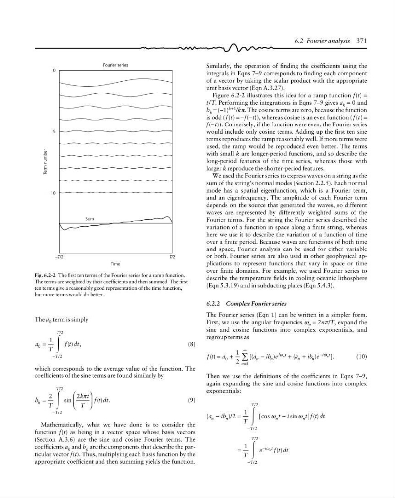
Figure 6.2-2 illustrates this idea for a ramp function f(t) =
t/T. Performing the integrations in Eqns 7–9 gives a k = 0 and
b k = (−1) k+1 /kπ. The cosine terms are zero, because the function
is odd ( f (t) = −f(−t)), whereas cosine is an even function ( f (t) =
f(−t)). Conversely, if the function were even, the Fourier series
would include only cosine terms. Adding up the first ten sine
terms reproduces the ramp reasonably well. If more terms were
used, the ramp would be reproduced even better. The terms
with small k are longer-period functions, and so describe the
long-period features of the time series, whereas those with
larger k reproduce the shorter-period features.
We used the Fourier series to express waves on a string as the
sum of the string’s normal modes (Section 2.2.5). Each normal
mode has a spatial eigenfunction, which is a Fourier term,
and an eigenfrequency. The amplitude of each Fourier term
depends on the source that generated the waves, so different
waves are represented by differently weighted sums of the
Fourier terms. For the string the Fourier series described the
variation of a function in space along a finite string, whereas
here we use it to describe the variation of a function of time
over a finite period. Because waves are functions of both time
and space, Fourier analysis can be used for either variable
or both. Fourier series are also used in other geophysical applications to represent functions that vary in space or time
over finite domains. For example, we used Fourier series to
describe the temperature fields in cooling oceanic lithosphere
(Eqn 5.3.19) and in subducting plates (Eqn 5.4.3).
6.2.2 Complex Fourier series
The Fourier series (Eqn 1) can be written in a simpler form.
First, we use the angular frequencies ω n = 2nπ/T, expand the
sine and cosine functions into complex exponentials, and
regroup terms as
f t a
a
ib e
a
ib e
n
n
n
i t
n
n
i t
n
n
( )
[(
)
(
)
].
=
+
−
+
+
=
∞
−
∑
0
1
1
2
ω
ω
(10)
Then we use the definitions of the coefficients in Eqns 7–9,
again expanding the sine and cosine functions into complex
exponentials:
(
)/
[cos
sin
] ( )
/
/
a
ib
T
t i
t f t dt
n
n
T
T
n
n
−
=
−
−
2
1
2
2
Ύ
ω
ω
=
−
−
( )
/
/
1
2
2
T
e
f t dt
T
T
i t
n
Ύ
ω
6.2 Fourier analysis 371
Term number
0
5
10
T/2
Time
–T/2
Fourier series
Sum
Fig. 6.2-2 The first ten terms of the Fourier series for a ramp function.
The terms are weighted by their coefficients and then summed. The first
ten terms give a reasonably good representation of the time function,
but more terms would do better.
The a 0 term is simply
a
T
f t dt
T
T
0
2
2
1
( ) ,
/
/
=
−
Ύ
(8)
which corresponds to the average value of the function. The
coefficients of the sine terms are found similarly by
b
T
k t
T
f t dt
k
T
T
sin
( ) .
/
/
=
⎛
⎝
⎜
⎞
⎠
⎟
−
2
2
2
2
Ύ
π
(9)
Mathematically, what we have done is to consider the
function f(t) as being in a vector space whose basis vectors
(Section A.3.6) are the sine and cosine Fourier terms. The
coefficients a k and b k are the components that describe the particular vector f(t). Thus, multiplying each basis function by the
appropriate coefficient and then summing yields the function.
integrals in Eqns 7–9 corresponds to finding each component
of a vector by taking the scalar product with the appropriate
unit basis vector (Eqn A.3.27).
Figure 6.2-2 illustrates this idea for a ramp function f(t) =
t/T. Performing the integrations in Eqns 7–9 gives a k = 0 and
b k = (−1) k+1 /kπ. The cosine terms are zero, because the function
is odd ( f (t) = −f(−t)), whereas cosine is an even function ( f (t) =
f(−t)). Conversely, if the function were even, the Fourier series
would include only cosine terms. Adding up the first ten sine
terms reproduces the ramp reasonably well. If more terms were
used, the ramp would be reproduced even better. The terms
with small k are longer-period functions, and so describe the
long-period features of the time series, whereas those with
larger k reproduce the shorter-period features.
We used the Fourier series to express waves on a string as the
sum of the string’s normal modes (Section 2.2.5). Each normal
mode has a spatial eigenfunction, which is a Fourier term,
and an eigenfrequency. The amplitude of each Fourier term
depends on the source that generated the waves, so different
waves are represented by differently weighted sums of the
Fourier terms. For the string the Fourier series described the
variation of a function in space along a finite string, whereas
here we use it to describe the variation of a function of time
over a finite period. Because waves are functions of both time
and space, Fourier analysis can be used for either variable
or both. Fourier series are also used in other geophysical applications to represent functions that vary in space or time
over finite domains. For example, we used Fourier series to
describe the temperature fields in cooling oceanic lithosphere
(Eqn 5.3.19) and in subducting plates (Eqn 5.4.3).
6.2.2 Complex Fourier series
The Fourier series (Eqn 1) can be written in a simpler form.
First, we use the angular frequencies ω n = 2nπ/T, expand the
sine and cosine functions into complex exponentials, and
regroup terms as
f t a
a
ib e
a
ib e
n
n
n
i t
n
n
i t
n
n
( )
[(
)
(
)
].
=
+
−
+
+
=
∞
−
∑
0
1
1
2
ω
ω
(10)
Then we use the definitions of the coefficients in Eqns 7–9,
again expanding the sine and cosine functions into complex
exponentials:
(
)/
[cos
sin
] ( )
/
/
a
ib
T
t i
t f t dt
n
n
T
T
n
n
−
=
−
−
2
1
2
2
Ύ
ω
ω
=
−
−
( )
/
/
1
2
2
T
e
f t dt
T
T
i t
n
Ύ
ω
6.2 Fourier analysis 371
Term number
0
5
10
T/2
Time
–T/2
Fourier series
Sum
Fig. 6.2-2 The first ten terms of the Fourier series for a ramp function.
The terms are weighted by their coefficients and then summed. The first
ten terms give a reasonably good representation of the time function,
but more terms would do better.
The a 0 term is simply
a
T
f t dt
T
T
0
2
2
1
( ) ,
/
/
=
−
Ύ
(8)
which corresponds to the average value of the function. The
coefficients of the sine terms are found similarly by
b
T
k t
T
f t dt
k
T
T
sin
( ) .
/
/
=
⎛
⎝
⎜
⎞
⎠
⎟
−
2
2
2
2
Ύ
π
(9)
Mathematically, what we have done is to consider the
function f(t) as being in a vector space whose basis vectors
(Section A.3.6) are the sine and cosine Fourier terms. The
coefficients a k and b k are the components that describe the particular vector f(t). Thus, multiplying each basis function by the
appropriate coefficient and then summing yields the function.