

370 Seismograms as Signals
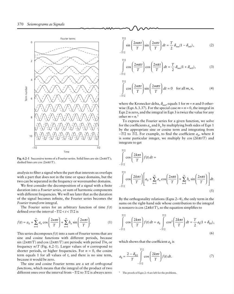
Fig. 6.2-1 Successive terms of a Fourier series. Solid lines are sin (2nπt/T );
dashed lines are cos (2nπt/T ).
1 The proofs of Eqns 2–4 are left for the problems.
analysis to filter a signal when the part that interests us overlaps
with a part that does not in the time or space domains, but the
two can be separated in the frequency or wavenumber domains.
We first consider the decomposition of a signal with a finite
duration into a Fourier series, or sum of harmonic components
with different frequencies. We will see later that as the duration
of the signal becomes infinite, the Fourier series becomes the
Fourier transform integral.
The Fourier series for an arbitrary function of time f (t)
defined over the interval −T/2 < t < T/2 is
f t a
a
n t
T
b
n t
T
n
n
n
n
( )
cos
sin
.
=
+
⎛
⎝
⎜
⎞
⎠
⎟ +
⎛
⎝
⎜
⎞
⎠
⎟
=
∞
=
∞
∑
∑
0
1
1
2
2
π
π
(1)
This series decomposes f(t) into a sum of Fourier terms that are
sine and cosine functions with different periods, because
sin (2nπt/T) and cos (2nπt /T ) are periodic with period T/n, or
frequency n/T (Fig. 6.2-1). Larger values of n correspond to
shorter periods, or higher frequencies. For n = 0, the cosine
term equals 1 for all values of t, and there is no sine term,
because it would be zero.
The sine and cosine Fourier terms are a set of orthogonal
functions, which means that the integral of the product of two
different ones over the interval from −T/2 to T/2 is always zero:
Ύ
−
⎛
⎝
⎜
⎞
⎠
⎟
⎛
⎝
⎜
⎞
⎠
⎟
=
−
T
T
mn
m
m t
T
n t
T
dt
T
/
/
sin
sin
(
),
2
2
0
2
2
2
1
π
π
δ
δ
(2)
Ύ
−
⎛
⎝
⎜
⎞
⎠
⎟
⎛
⎝
⎜
⎞
⎠
⎟
=
+
T
T
mn
m
m t
T
n t
T
dt
T
/
/
cos
cos
(
),
2
2
0
2
2
2
1
π
π
δ
δ
(3)
Ύ
−
⎛
⎝
⎜
⎞
⎠
⎟
⎛
⎝
⎜
⎞
⎠
⎟
=
T
T
n t
T
m t
T
dt
/
/
cos
sin
2
2
2
2
0
π
π
for all m, n,
(4)
where the Kronecker delta, δ mn , equals 1 for m = n and 0 otherwise (Eqn A.3.37). For the special case m = n = 0, the integral in
Eqn 2 is zero, and the integral in Eqn 3 is twice the value for any
other m = n.
1
To express the Fourier series for a given function, we solve
for the coefficients a n and b n by multiplying both sides of Eqn 1
by the appropriate sine or cosine term and integrating from
−T/2 to T/2. For example, to find the coefficient a k , where k
is some particular integer, we multiply by cos (2kπt/T) and
integrate to get
Ύ
−
⎛
⎝
⎜
⎞
⎠
⎟
=
T
T
k t
T
f t dt
/
/
cos
( )
2
2
2 π
Ύ
−
=
∞
=
∞
⎛
⎝
⎜
⎞
⎠
⎟
+
⎛
⎝
⎜
⎞
⎠
⎟ +
⎛
⎝
⎜
⎞
⎠
⎟
⎡
⎣
⎢
⎢
⎤
⎦
⎥
⎥
∑
∑
T
T
n
n
n
n
k t
T
a
a
n t
T
b
n t
T
dt
/
/
cos
cos
sin
.
2
2
0
1
1
2
2
2
π
π
π
(5)
By the orthogonality relations (Eqns 2–4), the only term in the
sums on the right-hand side whose contribution to the integral
is nonzero is cos (2πkt/T), so the equation simplifies to
Ύ
Ύ
−
−
⎛
⎝
⎜
⎞
⎠
⎟
=
⎛
⎝
⎜
⎞
⎠
⎟
=
+
T
T
k
T
T
k
k
k t
T
f t dt a
k t
T
dt
T a
/
/
/
/
cos
( )
cos
(
),
2
2
2
2
2
0
2
2
2
1
π
π
δ
(6)
which shows that the coefficient a k is
a
T
k t
T
f t dt
k
k
T
T
=
−
⎛
⎝
⎜
⎞
⎠
⎟
−
cos
( ) .
/
/
2
2
0
2
2
δ
π
Ύ
(7)
Term number
0
2
4
6
8
10
T/2
Time
–T/2
Fourier terms
Fig. 6.2-1 Successive terms of a Fourier series. Solid lines are sin (2nπt/T );
dashed lines are cos (2nπt/T ).
1 The proofs of Eqns 2–4 are left for the problems.
analysis to filter a signal when the part that interests us overlaps
with a part that does not in the time or space domains, but the
two can be separated in the frequency or wavenumber domains.
We first consider the decomposition of a signal with a finite
duration into a Fourier series, or sum of harmonic components
with different frequencies. We will see later that as the duration
of the signal becomes infinite, the Fourier series becomes the
Fourier transform integral.
The Fourier series for an arbitrary function of time f (t)
defined over the interval −T/2 < t < T/2 is
f t a
a
n t
T
b
n t
T
n
n
n
n
( )
cos
sin
.
=
+
⎛
⎝
⎜
⎞
⎠
⎟ +
⎛
⎝
⎜
⎞
⎠
⎟
=
∞
=
∞
∑
∑
0
1
1
2
2
π
π
(1)
This series decomposes f(t) into a sum of Fourier terms that are
sine and cosine functions with different periods, because
sin (2nπt/T) and cos (2nπt /T ) are periodic with period T/n, or
frequency n/T (Fig. 6.2-1). Larger values of n correspond to
shorter periods, or higher frequencies. For n = 0, the cosine
term equals 1 for all values of t, and there is no sine term,
because it would be zero.
The sine and cosine Fourier terms are a set of orthogonal
functions, which means that the integral of the product of two
different ones over the interval from −T/2 to T/2 is always zero:
Ύ
−
⎛
⎝
⎜
⎞
⎠
⎟
⎛
⎝
⎜
⎞
⎠
⎟
=
−
T
T
mn
m
m t
T
n t
T
dt
T
/
/
sin
sin
(
),
2
2
0
2
2
2
1
π
π
δ
δ
(2)
Ύ
−
⎛
⎝
⎜
⎞
⎠
⎟
⎛
⎝
⎜
⎞
⎠
⎟
=
+
T
T
mn
m
m t
T
n t
T
dt
T
/
/
cos
cos
(
),
2
2
0
2
2
2
1
π
π
δ
δ
(3)
Ύ
−
⎛
⎝
⎜
⎞
⎠
⎟
⎛
⎝
⎜
⎞
⎠
⎟
=
T
T
n t
T
m t
T
dt
/
/
cos
sin
2
2
2
2
0
π
π
for all m, n,
(4)
where the Kronecker delta, δ mn , equals 1 for m = n and 0 otherwise (Eqn A.3.37). For the special case m = n = 0, the integral in
Eqn 2 is zero, and the integral in Eqn 3 is twice the value for any
other m = n.
1
To express the Fourier series for a given function, we solve
for the coefficients a n and b n by multiplying both sides of Eqn 1
by the appropriate sine or cosine term and integrating from
−T/2 to T/2. For example, to find the coefficient a k , where k
is some particular integer, we multiply by cos (2kπt/T) and
integrate to get
Ύ
−
⎛
⎝
⎜
⎞
⎠
⎟
=
T
T
k t
T
f t dt
/
/
cos
( )
2
2
2 π
Ύ
−
=
∞
=
∞
⎛
⎝
⎜
⎞
⎠
⎟
+
⎛
⎝
⎜
⎞
⎠
⎟ +
⎛
⎝
⎜
⎞
⎠
⎟
⎡
⎣
⎢
⎢
⎤
⎦
⎥
⎥
∑
∑
T
T
n
n
n
n
k t
T
a
a
n t
T
b
n t
T
dt
/
/
cos
cos
sin
.
2
2
0
1
1
2
2
2
π
π
π
(5)
By the orthogonality relations (Eqns 2–4), the only term in the
sums on the right-hand side whose contribution to the integral
is nonzero is cos (2πkt/T), so the equation simplifies to
Ύ
Ύ
−
−
⎛
⎝
⎜
⎞
⎠
⎟
=
⎛
⎝
⎜
⎞
⎠
⎟
=
+
T
T
k
T
T
k
k
k t
T
f t dt a
k t
T
dt
T a
/
/
/
/
cos
( )
cos
(
),
2
2
2
2
2
0
2
2
2
1
π
π
δ
(6)
which shows that the coefficient a k is
a
T
k t
T
f t dt
k
k
T
T
=
−
⎛
⎝
⎜
⎞
⎠
⎟
−
cos
( ) .
/
/
2
2
0
2
2
δ
π
Ύ
(7)
Term number
0
2
4
6
8
10
T/2
Time
–T/2
Fourier terms