

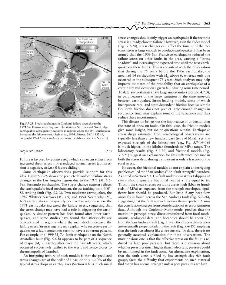
Fig. 5.7-25 Predicted changes in Coulomb failure stress due to the
1971 San Fernando earthquake. The Whittier Narrows and Northridge
earthquakes subsequently occurred in regions where the 1971 earthquake
increased the failure stress. (Stein et al., 1994. Science, 265, 1432–5,
copyright 1994 American Association for the Advancement of Science.)
faults
folds
S a n A n d re a s
20 km
1994
119°05’
33°55’
Pacific
L. A.
1987
1971−6
M ≥ 1
shocks
1971
−0.5
0.0
0.5
Coulomb stress
change (bars)
34°50’
117°50’
stress changes should only trigger an earthquake if the tectonic
stress is already close to failure. However, as in the slider model
(Fig. 5.7-24), stress changes can affect the time until the tectonic stress is large enough to produce earthquakes. It has been
argued that the 1906 San Francisco earthquake reduced the
failure stress on other faults in the area, causing a “stress
shadow” and increasing the expected time until the next earthquake on these faults. This is consistent with the observation
that during the 75 years before the 1906 earthquake, the
area had 14 earthquakes with M w above 6, whereas only one
occurred in the subsequent 75 years. Such analyses may help
improve estimates of the probability that an earthquake of a
certain size will occur on a given fault during some time period.
To date, such estimates have large uncertainties (Section 4.7.3),
in part because of the large variation in the time intervals
between earthquakes. Stress loading models, some of which
incorporate rate- and state-dependent friction because simple
Coulomb friction does not predict large enough changes in
recurrence time, may explain some of the variations and thus
reduce these uncertainties.
This discussion brings out the importance of understanding
the state of stress on faults. On this issue, the friction models
give some insight, but major questions remain. Earthquake
stress drops estimated from seismological observations are
typically less than a few hundred bars (tens of MPa). Yet, the
expected strength of the lithosphere (e.g., Fig. 5.7-14–16)
is much higher, in the kilobar (hundreds of MPa) range. The
laboratory results (Fig. 5.7-20) and frictional models (Fig.
5.7-21) suggest an explanation for this difference, because in
both the stress drop during a slip event is only a fraction of the
total stress.
However, the frictional models do not explain an intriguing
problem called the “San Andreas” or “fault strength” paradox.
As noted in Section 5.4.1, a fault under shear stress τ slipping at
rate v should generate fractional heat at a rate equal to τv.
Thus, if the shear stresses on faults are as high (kbar or hundreds of MPa) as expected from the strength envelopes, significant heat should be produced. But little if any heat flow
anomaly is found across the San Andreas fault (Fig. 5.7-26),
suggesting that the fault is much weaker than expected. A similar conclusion emerges from consideration of stress orientation
data. Although the Coulomb–Mohr model predicts that the
maximum principal stress directions inferred from focal mechanisms, geological data, and boreholes should be about 23°
from the San Andreas fault (Fig. 5.7-8), the observed directions
are essentially perpendicular to the fault (Fig. 5.6-19), implying
that the fault acts almost like a free surface. To date, there is no
generally accepted explanation for these observations. The
most obvious one is that the effective stress on the fault is reduced by high pore pressure, but there is discussion about
whether pressures much higher than hydrostatic pressure could
be maintained in the fault zone. An alternative explanation,
that the fault zone is filled by low-strength clay-rich fault
gouge, faces the difficulty that experiments on such material
find that it has normal strength unless pore pressures are high.
5.7 Faulting and deformation in the earth 363
∆σ f = ∆τ + µ∆σ.
(56)
Failure is favored by positive ∆σ f , which can occur either from
increased shear stress τ or a reduced normal stress (compression is negative, so ∆σ > 0 favors sliding).
Some earthquake observations provide support for this
idea. Figure 5.7-25 shows the predicted Coulomb failure stress
changes in the Los Angeles region due to the 1971 (M s 6.6)
San Fernando earthquake. The stress change pattern reflects
the earthquake’s focal mechanism, thrust faulting on a NW–
SE-striking fault (Fig. 5.2-3). Two moderate earthquakes, the
1987 Whittier Narrows (M L 5.9) and 1994 Northridge (M w
6.7) earthquakes subsequently occurred in regions where the
1971 earthquake increased the failure stress, suggesting that
the stress change may have had a role in triggering the earthquakes. A similar pattern has been found after other earthquakes, and some studies have found that aftershocks are
concentrated in regions where the mainshock increased the
failure stress. Stress triggering may explain why successive earthquakes on a fault sometimes seem to have a coherent pattern.
For example, the 1999 M s 7.4 Izmit earthquake on the North
Anatolian fault (Fig. 5.6-8) appears to be part of a sequence
of major (M s 7) earthquakes over the past 60 years, which
occurred successively further to the west, and hence closer to
the metropolis of Istanbul.
An intriguing feature of such models is that the predicted
stress changes are of the order of 1 bar, or only 1–10% of the
typical stress drops in earthquakes (Section 4.6.3). Such small
1971 San Fernando earthquake. The Whittier Narrows and Northridge
earthquakes subsequently occurred in regions where the 1971 earthquake
increased the failure stress. (Stein et al., 1994. Science, 265, 1432–5,
copyright 1994 American Association for the Advancement of Science.)
faults
folds
S a n A n d re a s
20 km
1994
119°05’
33°55’
Pacific
L. A.
1987
1971−6
M ≥ 1
shocks
1971
−0.5
0.0
0.5
Coulomb stress
change (bars)
34°50’
117°50’
stress changes should only trigger an earthquake if the tectonic
stress is already close to failure. However, as in the slider model
(Fig. 5.7-24), stress changes can affect the time until the tectonic stress is large enough to produce earthquakes. It has been
argued that the 1906 San Francisco earthquake reduced the
failure stress on other faults in the area, causing a “stress
shadow” and increasing the expected time until the next earthquake on these faults. This is consistent with the observation
that during the 75 years before the 1906 earthquake, the
area had 14 earthquakes with M w above 6, whereas only one
occurred in the subsequent 75 years. Such analyses may help
improve estimates of the probability that an earthquake of a
certain size will occur on a given fault during some time period.
To date, such estimates have large uncertainties (Section 4.7.3),
in part because of the large variation in the time intervals
between earthquakes. Stress loading models, some of which
incorporate rate- and state-dependent friction because simple
Coulomb friction does not predict large enough changes in
recurrence time, may explain some of the variations and thus
reduce these uncertainties.
This discussion brings out the importance of understanding
the state of stress on faults. On this issue, the friction models
give some insight, but major questions remain. Earthquake
stress drops estimated from seismological observations are
typically less than a few hundred bars (tens of MPa). Yet, the
expected strength of the lithosphere (e.g., Fig. 5.7-14–16)
is much higher, in the kilobar (hundreds of MPa) range. The
laboratory results (Fig. 5.7-20) and frictional models (Fig.
5.7-21) suggest an explanation for this difference, because in
both the stress drop during a slip event is only a fraction of the
total stress.
However, the frictional models do not explain an intriguing
problem called the “San Andreas” or “fault strength” paradox.
As noted in Section 5.4.1, a fault under shear stress τ slipping at
rate v should generate fractional heat at a rate equal to τv.
Thus, if the shear stresses on faults are as high (kbar or hundreds of MPa) as expected from the strength envelopes, significant heat should be produced. But little if any heat flow
anomaly is found across the San Andreas fault (Fig. 5.7-26),
suggesting that the fault is much weaker than expected. A similar conclusion emerges from consideration of stress orientation
data. Although the Coulomb–Mohr model predicts that the
maximum principal stress directions inferred from focal mechanisms, geological data, and boreholes should be about 23°
from the San Andreas fault (Fig. 5.7-8), the observed directions
are essentially perpendicular to the fault (Fig. 5.6-19), implying
that the fault acts almost like a free surface. To date, there is no
generally accepted explanation for these observations. The
most obvious one is that the effective stress on the fault is reduced by high pore pressure, but there is discussion about
whether pressures much higher than hydrostatic pressure could
be maintained in the fault zone. An alternative explanation,
that the fault zone is filled by low-strength clay-rich fault
gouge, faces the difficulty that experiments on such material
find that it has normal strength unless pore pressures are high.
5.7 Faulting and deformation in the earth 363
∆σ f = ∆τ + µ∆σ.
(56)
Failure is favored by positive ∆σ f , which can occur either from
increased shear stress τ or a reduced normal stress (compression is negative, so ∆σ > 0 favors sliding).
Some earthquake observations provide support for this
idea. Figure 5.7-25 shows the predicted Coulomb failure stress
changes in the Los Angeles region due to the 1971 (M s 6.6)
San Fernando earthquake. The stress change pattern reflects
the earthquake’s focal mechanism, thrust faulting on a NW–
SE-striking fault (Fig. 5.2-3). Two moderate earthquakes, the
1987 Whittier Narrows (M L 5.9) and 1994 Northridge (M w
6.7) earthquakes subsequently occurred in regions where the
1971 earthquake increased the failure stress, suggesting that
the stress change may have had a role in triggering the earthquakes. A similar pattern has been found after other earthquakes, and some studies have found that aftershocks are
concentrated in regions where the mainshock increased the
failure stress. Stress triggering may explain why successive earthquakes on a fault sometimes seem to have a coherent pattern.
For example, the 1999 M s 7.4 Izmit earthquake on the North
Anatolian fault (Fig. 5.6-8) appears to be part of a sequence
of major (M s 7) earthquakes over the past 60 years, which
occurred successively further to the west, and hence closer to
the metropolis of Istanbul.
An intriguing feature of such models is that the predicted
stress changes are of the order of 1 bar, or only 1–10% of the
typical stress drops in earthquakes (Section 4.6.3). Such small