

362 Seismology and Plate Tectonics
Depth (km)
D
0
10
20
30
A, B
Earthquake
Earthquake
Earthquake
B
A
C
B′
E
F
G
A to B
B to B′
B′ to C
C to D
D to E
E to F
F to G
300 days
instantaneous
2.5 min
4.2 days
1.9 yr
9.1 yr
82.5 yr
Time interval
T cy = 92.9 yr
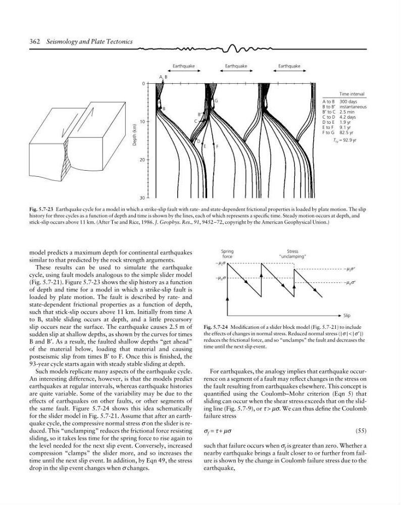
Fig. 5.7-23 Earthquake cycle for a model in which a strike-slip fault with rate- and state-dependent frictional properties is loaded by plate motion. The slip
history for three cycles as a function of depth and time is shown by the lines, each of which represents a specific time. Steady motion occurs at depth, and
stick-slip occurs above 11 km. (After Tse and Rice, 1986. J. Geophys. Res., 91, 9452–72, copyright by the American Geophysical Union.)
model predicts a maximum depth for continental earthquakes
similar to that predicted by the rock strength arguments.
These results can be used to simulate the earthquake
cycle, using fault models analogous to the simple slider model
(Fig. 5.7-21). Figure 5.7-23 shows the slip history as a function
of depth and time for a model in which a strike-slip fault is
loaded by plate motion. The fault is described by rate- and
state-dependent frictional properties as a function of depth,
such that stick-slip occurs above 11 km. Initially from time A
to B, stable sliding occurs at depth, and a little precursory
slip occurs near the surface. The earthquake causes 2.5 m of
sudden slip at shallow depths, as shown by the curves for times
B and B′. As a result, the faulted shallow depths “get ahead”
of the material below, loading that material and causing
postseismic slip from times B′ to F. Once this is finished, the
93-year cycle starts again with steady stable sliding at depth.
Such models replicate many aspects of the earthquake cycle.
An interesting difference, however, is that the models predict
earthquakes at regular intervals, whereas earthquake histories
are quite variable. Some of the variability may be due to the
effects of earthquakes on other faults, or other segments of
the same fault. Figure 5.7-24 shows this idea schematically
for the slider model in Fig. 5.7-21. Assume that after an earthquake cycle, the compressive normal stress σ on the slider is reduced. This “unclamping” reduces the frictional force resisting
sliding, so it takes less time for the spring force to rise again to
the level needed for the next slip event. Conversely, increased
compression “clamps” the slider more, and so increases the
time until the next slip event. In addition, by Eqn 49, the stress
drop in the slip event changes when σ changes.
Stress
“unclamping”
µ σ
d
−
µ σ
s
−
µ σ
d
−
′
µ σ
s
−
′
Slip
Spring
force
Fig. 5.7-24 Modification of a slider block model (Fig. 5.7-21) to include
the effects of changes in normal stress. Reduced normal stress ( | σ | < | σ ′ |)
reduces the frictional force, and so “unclamps” the fault and decreases the
time until the next slip event.
For earthquakes, the analogy implies that earthquake occurrence on a segment of a fault may reflect changes in the stress on
the fault resulting from earthquakes elsewhere. This concept is
quantified using the Coulomb–Mohr criterion (Eqn 5) that
sliding can occur when the shear stress exceeds that on the sliding line (Fig. 5.7-9), or τ > µσ. We can thus define the Coulomb
failure stress
σ f = τ + µσ
(55)
such that failure occurs when σ f is greater than zero. Whether a
nearby earthquake brings a fault closer to or further from failure is shown by the change in Coulomb failure stress due to the
earthquake,
Depth (km)
D
0
10
20
30
A, B
Earthquake
Earthquake
Earthquake
B
A
C
B′
E
F
G
A to B
B to B′
B′ to C
C to D
D to E
E to F
F to G
300 days
instantaneous
2.5 min
4.2 days
1.9 yr
9.1 yr
82.5 yr
Time interval
T cy = 92.9 yr
Fig. 5.7-23 Earthquake cycle for a model in which a strike-slip fault with rate- and state-dependent frictional properties is loaded by plate motion. The slip
history for three cycles as a function of depth and time is shown by the lines, each of which represents a specific time. Steady motion occurs at depth, and
stick-slip occurs above 11 km. (After Tse and Rice, 1986. J. Geophys. Res., 91, 9452–72, copyright by the American Geophysical Union.)
model predicts a maximum depth for continental earthquakes
similar to that predicted by the rock strength arguments.
These results can be used to simulate the earthquake
cycle, using fault models analogous to the simple slider model
(Fig. 5.7-21). Figure 5.7-23 shows the slip history as a function
of depth and time for a model in which a strike-slip fault is
loaded by plate motion. The fault is described by rate- and
state-dependent frictional properties as a function of depth,
such that stick-slip occurs above 11 km. Initially from time A
to B, stable sliding occurs at depth, and a little precursory
slip occurs near the surface. The earthquake causes 2.5 m of
sudden slip at shallow depths, as shown by the curves for times
B and B′. As a result, the faulted shallow depths “get ahead”
of the material below, loading that material and causing
postseismic slip from times B′ to F. Once this is finished, the
93-year cycle starts again with steady stable sliding at depth.
Such models replicate many aspects of the earthquake cycle.
An interesting difference, however, is that the models predict
earthquakes at regular intervals, whereas earthquake histories
are quite variable. Some of the variability may be due to the
effects of earthquakes on other faults, or other segments of
the same fault. Figure 5.7-24 shows this idea schematically
for the slider model in Fig. 5.7-21. Assume that after an earthquake cycle, the compressive normal stress σ on the slider is reduced. This “unclamping” reduces the frictional force resisting
sliding, so it takes less time for the spring force to rise again to
the level needed for the next slip event. Conversely, increased
compression “clamps” the slider more, and so increases the
time until the next slip event. In addition, by Eqn 49, the stress
drop in the slip event changes when σ changes.
Stress
“unclamping”
µ σ
d
−
µ σ
s
−
µ σ
d
−
′
µ σ
s
−
′
Slip
Spring
force
Fig. 5.7-24 Modification of a slider block model (Fig. 5.7-21) to include
the effects of changes in normal stress. Reduced normal stress ( | σ | < | σ ′ |)
reduces the frictional force, and so “unclamps” the fault and decreases the
time until the next slip event.
For earthquakes, the analogy implies that earthquake occurrence on a segment of a fault may reflect changes in the stress on
the fault resulting from earthquakes elsewhere. This concept is
quantified using the Coulomb–Mohr criterion (Eqn 5) that
sliding can occur when the shear stress exceeds that on the sliding line (Fig. 5.7-9), or τ > µσ. We can thus define the Coulomb
failure stress
σ f = τ + µσ
(55)
such that failure occurs when σ f is greater than zero. Whether a
nearby earthquake brings a fault closer to or further from failure is shown by the change in Coulomb failure stress due to the
earthquake,