

Failure angle
2θ f
τ
τ o
σ
Failure line
µσ
τ = −
o
τ
Sliding angles
2 s 1
θ
2 s 2
θ
= −
Sliding line
µσ
τ
At this point, it is worth noting other complexities. Both the
failure and sliding curves may be more complicated than
straight lines. These curves, known as Mohr envelopes, can be
derived from experiments at various values of stress. Additional complexity comes from the fact that water and other
fluids are often present in rocks, especially in the upper crust.
The fluid pressure, known as the pore pressure, reduces the
effect of the normal stress and allows sliding to take place at
lower shear stresses. This effect is modeled by replacing the
normal stress σ with O = σ − P f , known as the effective normal
stress, where P f is the pore fluid pressure. 2 Because the pore
pressure is defined as negative, the effective normal stress is
reduced (less compressive). Similarly, effective principal stresses
taking into account pore pressure,
O 1 = σ 1 − P f and O 2 = σ 2 − P f ,
(16)
are used in the fracture theory.
The relations we have discussed can be used to estimate the
maximum stresses that the crust can support. Laboratory experiments (Fig. 5.7-10) for sliding on existing faults in a variety
of rock types find relations sometimes called Byerlee’s law:
τ ≈ −0.85O, |O| < 200 MPa
τ ≈ 50 − 0.6O, |O| > 200 MPa.
(17)
These relations, written in terms of the normal and shear
stresses on a fault, can be used to infer the principal stress as
a function of depth. To do so, we write the minimum compressive stress as σ 3 , because we are in three dimensions. We
assume that the crust contains faults of all orientations, and
that the stresses cannot exceed the point where Mohr’s circle is
tangent to the frictional sliding line, or else sliding will occur
(Fig. 5.7-11). At shallow depths where |O| < 200 MPa, Eqn 17
shows that τ 0 = 0. Thus Eqn 13, the relation between the
stresses when fracture occurs, yields
O 1 = O 3 tan 2 θ s .
(18)
Using Eqn 7 for the case of frictional sliding,
θ s = α /2 + 45°,
(19)
and the values in Eqn 17 give
µ = tan α = 0.85, α ≈ 41°, θ s ≈ 66°, tan 2 66° ≈ 5,
(20)
so the stresses are related by
O 1 ≈ 5O 3 .
(21)
At greater depths, where |O| > 200 MPa, α ≈ 31° and θ s = 60.5°,
so the stresses are related by
O 1 ≈ −175 + 3.1O 3 .
(22)
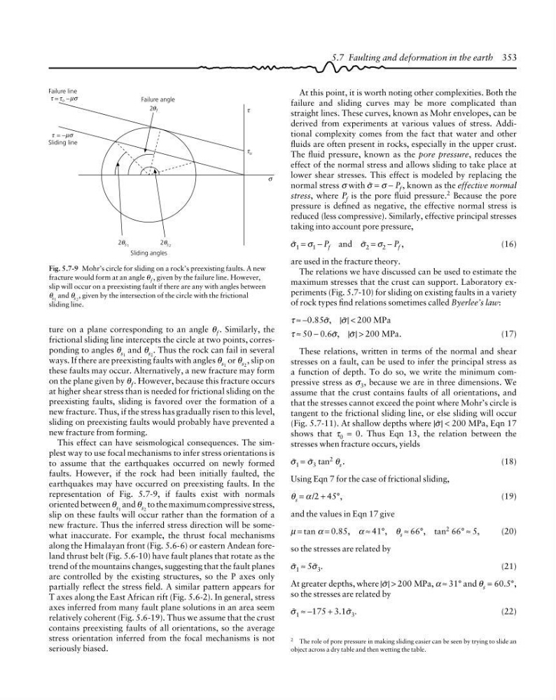
Fig. 5.7-9 Mohr’s circle for sliding on a rock’s preexisting faults. A new
fracture would form at an angle θ f , given by the failure line. However,
slip will occur on a preexisting fault if there are any with angles between
θ s1 and θ s2 , given by the intersection of the circle with the frictional
sliding line.
2 The role of pore pressure in making sliding easier can be seen by trying to slide an
object across a dry table and then wetting the table.
5.7 Faulting and deformation in the earth 353
ture on a plane corresponding to an angle θ f . Similarly, the
frictional sliding line intercepts the circle at two points, corresponding to angles θ s 1 and θ s 2 . Thus the rock can fail in several
ways. If there are preexisting faults with angles θ s 1 or θ s 2 , slip on
these faults may occur. Alternatively, a new fracture may form
on the plane given by θ f . However, because this fracture occurs
at higher shear stress than is needed for frictional sliding on the
preexisting faults, sliding is favored over the formation of a
new fracture. Thus, if the stress has gradually risen to this level,
sliding on preexisting faults would probably have prevented a
new fracture from forming.
This effect can have seismological consequences. The simplest way to use focal mechanisms to infer stress orientations is
to assume that the earthquakes occurred on newly formed
faults. However, if the rock had been initially faulted, the
earthquakes may have occurred on preexisting faults. In the
representation of Fig. 5.7-9, if faults exist with normals
oriented between θ s 1 and θ s 2 to the maximum compressive stress,
slip on these faults will occur rather than the formation of a
new fracture. Thus the inferred stress direction will be somewhat inaccurate. For example, the thrust focal mechanisms
along the Himalayan front (Fig. 5.6-6) or eastern Andean foreland thrust belt (Fig. 5.6-10) have fault planes that rotate as the
trend of the mountains changes, suggesting that the fault planes
are controlled by the existing structures, so the P axes only
partially reflect the stress field. A similar pattern appears for
T axes along the East African rift (Fig. 5.6-2). In general, stress
axes inferred from many fault plane solutions in an area seem
relatively coherent (Fig. 5.6-19). Thus we assume that the crust
contains preexisting faults of all orientations, so the average
stress orientation inferred from the focal mechanisms is not
seriously biased.
2θ f
τ
τ o
σ
Failure line
µσ
τ = −
o
τ
Sliding angles
2 s 1
θ
2 s 2
θ
= −
Sliding line
µσ
τ
At this point, it is worth noting other complexities. Both the
failure and sliding curves may be more complicated than
straight lines. These curves, known as Mohr envelopes, can be
derived from experiments at various values of stress. Additional complexity comes from the fact that water and other
fluids are often present in rocks, especially in the upper crust.
The fluid pressure, known as the pore pressure, reduces the
effect of the normal stress and allows sliding to take place at
lower shear stresses. This effect is modeled by replacing the
normal stress σ with O = σ − P f , known as the effective normal
stress, where P f is the pore fluid pressure. 2 Because the pore
pressure is defined as negative, the effective normal stress is
reduced (less compressive). Similarly, effective principal stresses
taking into account pore pressure,
O 1 = σ 1 − P f and O 2 = σ 2 − P f ,
(16)
are used in the fracture theory.
The relations we have discussed can be used to estimate the
maximum stresses that the crust can support. Laboratory experiments (Fig. 5.7-10) for sliding on existing faults in a variety
of rock types find relations sometimes called Byerlee’s law:
τ ≈ −0.85O, |O| < 200 MPa
τ ≈ 50 − 0.6O, |O| > 200 MPa.
(17)
These relations, written in terms of the normal and shear
stresses on a fault, can be used to infer the principal stress as
a function of depth. To do so, we write the minimum compressive stress as σ 3 , because we are in three dimensions. We
assume that the crust contains faults of all orientations, and
that the stresses cannot exceed the point where Mohr’s circle is
tangent to the frictional sliding line, or else sliding will occur
(Fig. 5.7-11). At shallow depths where |O| < 200 MPa, Eqn 17
shows that τ 0 = 0. Thus Eqn 13, the relation between the
stresses when fracture occurs, yields
O 1 = O 3 tan 2 θ s .
(18)
Using Eqn 7 for the case of frictional sliding,
θ s = α /2 + 45°,
(19)
and the values in Eqn 17 give
µ = tan α = 0.85, α ≈ 41°, θ s ≈ 66°, tan 2 66° ≈ 5,
(20)
so the stresses are related by
O 1 ≈ 5O 3 .
(21)
At greater depths, where |O| > 200 MPa, α ≈ 31° and θ s = 60.5°,
so the stresses are related by
O 1 ≈ −175 + 3.1O 3 .
(22)
Fig. 5.7-9 Mohr’s circle for sliding on a rock’s preexisting faults. A new
fracture would form at an angle θ f , given by the failure line. However,
slip will occur on a preexisting fault if there are any with angles between
θ s1 and θ s2 , given by the intersection of the circle with the frictional
sliding line.
2 The role of pore pressure in making sliding easier can be seen by trying to slide an
object across a dry table and then wetting the table.
5.7 Faulting and deformation in the earth 353
ture on a plane corresponding to an angle θ f . Similarly, the
frictional sliding line intercepts the circle at two points, corresponding to angles θ s 1 and θ s 2 . Thus the rock can fail in several
ways. If there are preexisting faults with angles θ s 1 or θ s 2 , slip on
these faults may occur. Alternatively, a new fracture may form
on the plane given by θ f . However, because this fracture occurs
at higher shear stress than is needed for frictional sliding on the
preexisting faults, sliding is favored over the formation of a
new fracture. Thus, if the stress has gradually risen to this level,
sliding on preexisting faults would probably have prevented a
new fracture from forming.
This effect can have seismological consequences. The simplest way to use focal mechanisms to infer stress orientations is
to assume that the earthquakes occurred on newly formed
faults. However, if the rock had been initially faulted, the
earthquakes may have occurred on preexisting faults. In the
representation of Fig. 5.7-9, if faults exist with normals
oriented between θ s 1 and θ s 2 to the maximum compressive stress,
slip on these faults will occur rather than the formation of a
new fracture. Thus the inferred stress direction will be somewhat inaccurate. For example, the thrust focal mechanisms
along the Himalayan front (Fig. 5.6-6) or eastern Andean foreland thrust belt (Fig. 5.6-10) have fault planes that rotate as the
trend of the mountains changes, suggesting that the fault planes
are controlled by the existing structures, so the P axes only
partially reflect the stress field. A similar pattern appears for
T axes along the East African rift (Fig. 5.6-2). In general, stress
axes inferred from many fault plane solutions in an area seem
relatively coherent (Fig. 5.6-19). Thus we assume that the crust
contains preexisting faults of all orientations, so the average
stress orientation inferred from the focal mechanisms is not
seriously biased.