

Stress (MPa)
30
20
10
0
10
Drag coefficient
(MPa/(m/yr) )
compression
extension
0
400
300
200
100
Stress (MPa)
30
20
10
0
10
0
Drag coefficient
(MPa/(m/yr) )
compression
extension
50
100
150
0
4
3
2
1
Age (Myr)
6 Viscosity, defined in Section 5.7, is given in cgs units as poise (dyn-s/cm
2 ) or in SI
units as Pascal-seconds (1 poise = 0.1 Pa-s).
Fig. 5.5-9 Intraplate stress in the spreading direction as a function of
lithospheric age computed for several values of ridge strength. The age of
the transition from ridge-normal extension to compression increases with
the strength of the ridge. (Wiens and Stein, 1984. J. Geophys. Res., 89, 11,
442–64, copyright by the American Geophysical Union.)
20
10
0
−10
−20
Stress (MPa)
Halfspace model
Plate velocity = 5 cm/yr
Drag coefficient = 3 MPa/(m/yr)
compression
extension
20
40
60
0
30
20
10
Age (Myr)
Ridge strength (MPa)
5.5 Oceanic intraplate earthquakes and tectonics 331
zone (Fig. 5.5-5) that are generally consistent with the focal
mechanisms and the folding seen in gravity and seismic reflection data.
5.5.3 Constraints on mantle viscosity
The last section’s analysis relating earthquake mechanisms
to drag at the base of the lithosphere also gives insight into the
viscosity of the mantle. The viscosity,
6 the proportionality
constant between shear stress and the strain rate (or velocity
gradient), controls how the mantle flows in response to applied
stress, and is thus crucial for mantle convection. If the drag on
the base of a plate is due to motion over the viscous mantle,
compressive earthquake mechanisms in old lithosphere constrain the viscosity.
Consider a simple two-dimensional geometry where mass
flux due to the moving plate is balanced by a return flow at
depth (Fig. 5.5-11, top). The drag coefficient is proportional to
the viscosity and inversely proportional to the flow depth. Figure 5.5-12 shows that the basal drag constraint from the focal
mechanism data, C ≤ 4 MPa/(m/yr), requires an average mantle
viscosity less than 2 × 10 20 poise if flow occurs to a depth of
700 km in the upper mantle, or 10 21 poise if flow occurs in the
entire mantle. These values are lower than the 1–5 × 10 22 poise
typically estimated from glacial rebound, earth rotation, and
satellite orbits.
This discrepancy can be reconciled by assuming that the plate
is underlain by a thin, low-viscosity asthenosphere (Fig. 5.5-11,
bottom). The low-viscosity layer, in which only a fraction of the
return flow occurs, decouples the plates from the underlying
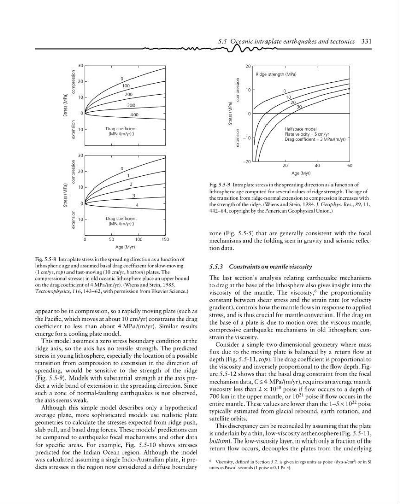
Fig. 5.5-8 Intraplate stress in the spreading direction as a function of
lithospheric age and assumed basal drag coefficient for slow-moving
(1 cm/yr, top) and fast-moving (10 cm/yr, bottom) plates. The
compressional stresses in old oceanic lithosphere place an upper bound
on the drag coefficient of 4 MPa/(m/yr). (Wiens and Stein, 1985.
Tectonophysics, 116, 143–62, with permission from Elsevier Science.)
appear to be in compression, so a rapidly moving plate (such as
the Pacific, which moves at about 10 cm/yr) constrains the drag
coefficient to less than about 4 MPa/(m/yr). Similar results
emerge for a cooling plate model.
This model assumes a zero stress boundary condition at the
ridge axis, so the axis has no tensile strength. The predicted
stress in young lithosphere, especially the location of a possible
transition from compression to extension in the direction of
spreading, would be sensitive to the strength of the ridge
(Fig. 5.5-9). Models with substantial strength at the axis predict a wide band of extension in the spreading direction. Since
such a zone of normal-faulting earthquakes is not observed,
the axis seems weak.
Although this simple model describes only a hypothetical
average plate, more sophisticated models use realistic plate
geometries to calculate the stresses expected from ridge push,
slab pull, and basal drag forces. These models’ predictions can
be compared to earthquake focal mechanisms and other data
for specific areas. For example, Fig. 5.5-10 shows stresses
predicted for the Indian Ocean region. Although the model
was calculated assuming a single Indo-Australian plate, it predicts stresses in the region now considered a diffuse boundary
30
20
10
0
10
Drag coefficient
(MPa/(m/yr) )
compression
extension
0
400
300
200
100
Stress (MPa)
30
20
10
0
10
0
Drag coefficient
(MPa/(m/yr) )
compression
extension
50
100
150
0
4
3
2
1
Age (Myr)
6 Viscosity, defined in Section 5.7, is given in cgs units as poise (dyn-s/cm
2 ) or in SI
units as Pascal-seconds (1 poise = 0.1 Pa-s).
Fig. 5.5-9 Intraplate stress in the spreading direction as a function of
lithospheric age computed for several values of ridge strength. The age of
the transition from ridge-normal extension to compression increases with
the strength of the ridge. (Wiens and Stein, 1984. J. Geophys. Res., 89, 11,
442–64, copyright by the American Geophysical Union.)
20
10
0
−10
−20
Stress (MPa)
Halfspace model
Plate velocity = 5 cm/yr
Drag coefficient = 3 MPa/(m/yr)
compression
extension
20
40
60
0
30
20
10
Age (Myr)
Ridge strength (MPa)
5.5 Oceanic intraplate earthquakes and tectonics 331
zone (Fig. 5.5-5) that are generally consistent with the focal
mechanisms and the folding seen in gravity and seismic reflection data.
5.5.3 Constraints on mantle viscosity
The last section’s analysis relating earthquake mechanisms
to drag at the base of the lithosphere also gives insight into the
viscosity of the mantle. The viscosity,
6 the proportionality
constant between shear stress and the strain rate (or velocity
gradient), controls how the mantle flows in response to applied
stress, and is thus crucial for mantle convection. If the drag on
the base of a plate is due to motion over the viscous mantle,
compressive earthquake mechanisms in old lithosphere constrain the viscosity.
Consider a simple two-dimensional geometry where mass
flux due to the moving plate is balanced by a return flow at
depth (Fig. 5.5-11, top). The drag coefficient is proportional to
the viscosity and inversely proportional to the flow depth. Figure 5.5-12 shows that the basal drag constraint from the focal
mechanism data, C ≤ 4 MPa/(m/yr), requires an average mantle
viscosity less than 2 × 10 20 poise if flow occurs to a depth of
700 km in the upper mantle, or 10 21 poise if flow occurs in the
entire mantle. These values are lower than the 1–5 × 10 22 poise
typically estimated from glacial rebound, earth rotation, and
satellite orbits.
This discrepancy can be reconciled by assuming that the plate
is underlain by a thin, low-viscosity asthenosphere (Fig. 5.5-11,
bottom). The low-viscosity layer, in which only a fraction of the
return flow occurs, decouples the plates from the underlying
Fig. 5.5-8 Intraplate stress in the spreading direction as a function of
lithospheric age and assumed basal drag coefficient for slow-moving
(1 cm/yr, top) and fast-moving (10 cm/yr, bottom) plates. The
compressional stresses in old oceanic lithosphere place an upper bound
on the drag coefficient of 4 MPa/(m/yr). (Wiens and Stein, 1985.
Tectonophysics, 116, 143–62, with permission from Elsevier Science.)
appear to be in compression, so a rapidly moving plate (such as
the Pacific, which moves at about 10 cm/yr) constrains the drag
coefficient to less than about 4 MPa/(m/yr). Similar results
emerge for a cooling plate model.
This model assumes a zero stress boundary condition at the
ridge axis, so the axis has no tensile strength. The predicted
stress in young lithosphere, especially the location of a possible
transition from compression to extension in the direction of
spreading, would be sensitive to the strength of the ridge
(Fig. 5.5-9). Models with substantial strength at the axis predict a wide band of extension in the spreading direction. Since
such a zone of normal-faulting earthquakes is not observed,
the axis seems weak.
Although this simple model describes only a hypothetical
average plate, more sophisticated models use realistic plate
geometries to calculate the stresses expected from ridge push,
slab pull, and basal drag forces. These models’ predictions can
be compared to earthquake focal mechanisms and other data
for specific areas. For example, Fig. 5.5-10 shows stresses
predicted for the Indian Ocean region. Although the model
was calculated assuming a single Indo-Australian plate, it predicts stresses in the region now considered a diffuse boundary