

314 Seismology and Plate Tectonics
a. Body force
z = 0
ρgz
z = L
Free
T = 0
Fixed
T = − gL
c. Compression
b. Tension
Fixed
ρ
T = gL
ρ
Free
T = 0
d. Both
Fixed
T = gL /2
ρ
T = − gL /2
ρ
Fixed
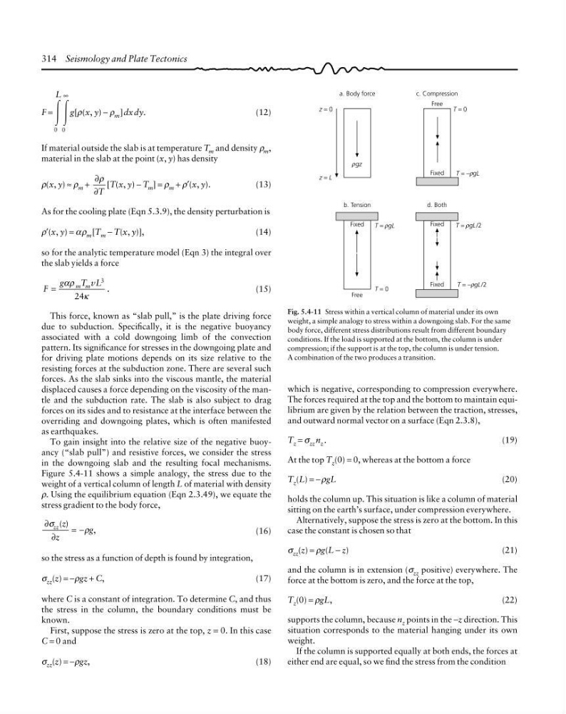
Fig. 5.4-11 Stress within a vertical column of material under its own
weight, a simple analogy to stress within a downgoing slab. For the same
body force, different stress distributions result from different boundary
conditions. If the load is supported at the bottom, the column is under
compression; if the support is at the top, the column is under tension.
A combination of the two produces a transition.
F =
ΎΎ
0 0
L ∞
g[ρ(x, y) − ρ m ]dxdy.
(12)
If material outside the slab is at temperature T m and density ρ m ,
material in the slab at the point (x, y) has density
ρ(x, y) ≈ ρ m +
∂
∂
ρ
T
[T(x, y) − T m ] = ρ m + ρ′(x, y).
(13)
As for the cooling plate (Eqn 5.3.9), the density perturbation is
ρ′(x, y) = αρ m [T m − T(x, y)],
(14)
so for the analytic temperature model (Eqn 3) the integral over
the slab yields a force
F
g
T vL
m m
.
=
αρ
κ
3
24
(15)
This force, known as “slab pull,” is the plate driving force
due to subduction. Specifically, it is the negative buoyancy
associated with a cold downgoing limb of the convection
pattern. Its significance for stresses in the downgoing plate and
for driving plate motions depends on its size relative to the
resisting forces at the subduction zone. There are several such
forces. As the slab sinks into the viscous mantle, the material
displaced causes a force depending on the viscosity of the mantle and the subduction rate. The slab is also subject to drag
forces on its sides and to resistance at the interface between the
overriding and downgoing plates, which is often manifested
as earthquakes.
To gain insight into the relative size of the negative buoyancy (“slab pull”) and resistive forces, we consider the stress
in the downgoing slab and the resulting focal mechanisms.
Figure 5.4-11 shows a simple analogy, the stress due to the
weight of a vertical column of length L of material with density
ρ. Using the equilibrium equation (Eqn 2.3.49), we equate the
stress gradient to the body force,
∂
∂
σ
ρ
zz z
z
g
( )
,
= −
(16)
so the stress as a function of depth is found by integration,
σ zz (z) = −ρgz + C,
(17)
where C is a constant of integration. To determine C, and thus
the stress in the column, the boundary conditions must be
known.
First, suppose the stress is zero at the top, z = 0. In this case
C = 0 and
σ zz (z) = −ρgz,
(18)
which is negative, corresponding to compression everywhere.
The forces required at the top and the bottom to maintain equilibrium are given by the relation between the traction, stresses,
and outward normal vector on a surface (Eqn 2.3.8),
T z = σ zz n z .
(19)
At the top T z (0) = 0, whereas at the bottom a force
T z (L) = −ρgL
(20)
holds the column up. This situation is like a column of material
sitting on the earth’s surface, under compression everywhere.
Alternatively, suppose the stress is zero at the bottom. In this
case the constant is chosen so that
σ zz (z) = ρg(L − z)
(21)
and the column is in extension (σ zz positive) everywhere. The
force at the bottom is zero, and the force at the top,
T z (0) = ρgL,
(22)
supports the column, because n z points in the −z direction. This
situation corresponds to the material hanging under its own
weight.
If the column is supported equally at both ends, the forces at
either end are equal, so we find the stress from the condition
a. Body force
z = 0
ρgz
z = L
Free
T = 0
Fixed
T = − gL
c. Compression
b. Tension
Fixed
ρ
T = gL
ρ
Free
T = 0
d. Both
Fixed
T = gL /2
ρ
T = − gL /2
ρ
Fixed
Fig. 5.4-11 Stress within a vertical column of material under its own
weight, a simple analogy to stress within a downgoing slab. For the same
body force, different stress distributions result from different boundary
conditions. If the load is supported at the bottom, the column is under
compression; if the support is at the top, the column is under tension.
A combination of the two produces a transition.
F =
ΎΎ
0 0
L ∞
g[ρ(x, y) − ρ m ]dxdy.
(12)
If material outside the slab is at temperature T m and density ρ m ,
material in the slab at the point (x, y) has density
ρ(x, y) ≈ ρ m +
∂
∂
ρ
T
[T(x, y) − T m ] = ρ m + ρ′(x, y).
(13)
As for the cooling plate (Eqn 5.3.9), the density perturbation is
ρ′(x, y) = αρ m [T m − T(x, y)],
(14)
so for the analytic temperature model (Eqn 3) the integral over
the slab yields a force
F
g
T vL
m m
.
=
αρ
κ
3
24
(15)
This force, known as “slab pull,” is the plate driving force
due to subduction. Specifically, it is the negative buoyancy
associated with a cold downgoing limb of the convection
pattern. Its significance for stresses in the downgoing plate and
for driving plate motions depends on its size relative to the
resisting forces at the subduction zone. There are several such
forces. As the slab sinks into the viscous mantle, the material
displaced causes a force depending on the viscosity of the mantle and the subduction rate. The slab is also subject to drag
forces on its sides and to resistance at the interface between the
overriding and downgoing plates, which is often manifested
as earthquakes.
To gain insight into the relative size of the negative buoyancy (“slab pull”) and resistive forces, we consider the stress
in the downgoing slab and the resulting focal mechanisms.
Figure 5.4-11 shows a simple analogy, the stress due to the
weight of a vertical column of length L of material with density
ρ. Using the equilibrium equation (Eqn 2.3.49), we equate the
stress gradient to the body force,
∂
∂
σ
ρ
zz z
z
g
( )
,
= −
(16)
so the stress as a function of depth is found by integration,
σ zz (z) = −ρgz + C,
(17)
where C is a constant of integration. To determine C, and thus
the stress in the column, the boundary conditions must be
known.
First, suppose the stress is zero at the top, z = 0. In this case
C = 0 and
σ zz (z) = −ρgz,
(18)
which is negative, corresponding to compression everywhere.
The forces required at the top and the bottom to maintain equilibrium are given by the relation between the traction, stresses,
and outward normal vector on a surface (Eqn 2.3.8),
T z = σ zz n z .
(19)
At the top T z (0) = 0, whereas at the bottom a force
T z (L) = −ρgL
(20)
holds the column up. This situation is like a column of material
sitting on the earth’s surface, under compression everywhere.
Alternatively, suppose the stress is zero at the bottom. In this
case the constant is chosen so that
σ zz (z) = ρg(L − z)
(21)
and the column is in extension (σ zz positive) everywhere. The
force at the bottom is zero, and the force at the top,
T z (0) = ρgL,
(22)
supports the column, because n z points in the −z direction. This
situation corresponds to the material hanging under its own
weight.
If the column is supported equally at both ends, the forces at
either end are equal, so we find the stress from the condition