

1000°
0
200
400
600
800
1000
Depth (km)
500°
200
400
600
800
1000
Isothermal mantle
Distance (km)
v
L
x
y
T = 0
T = T m
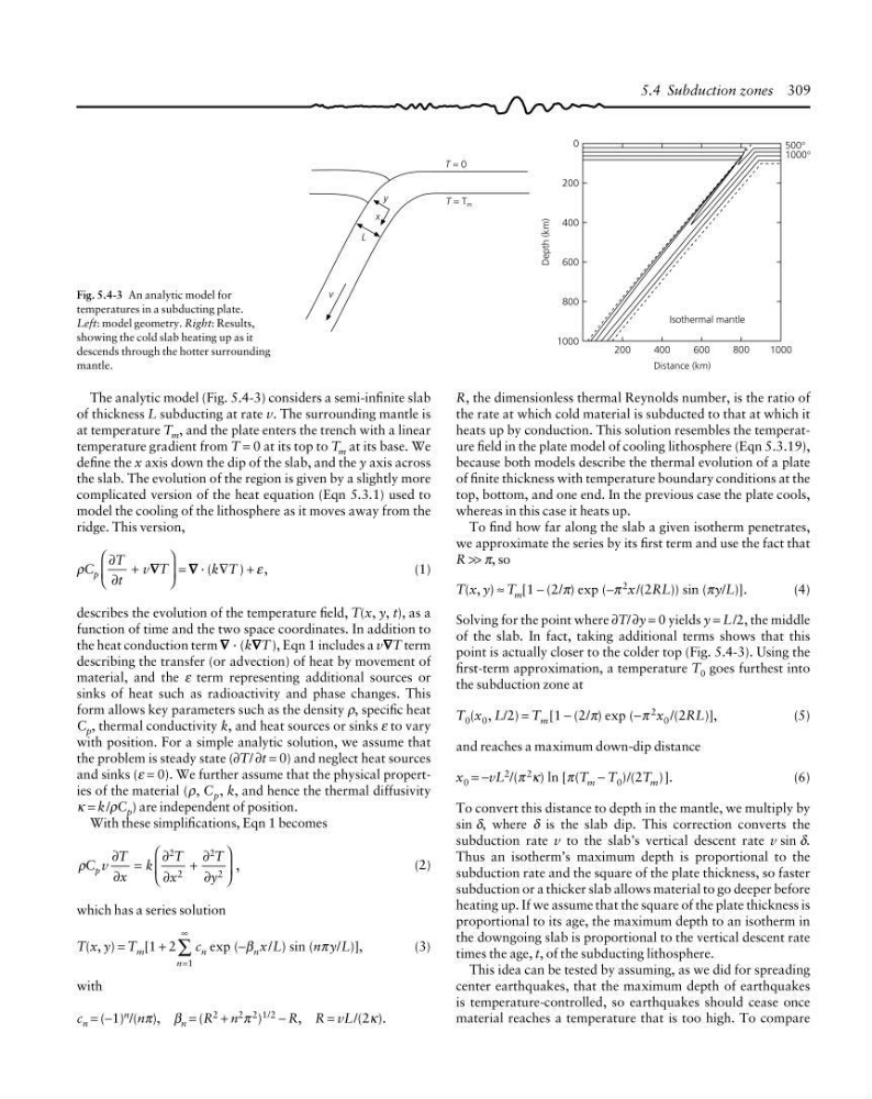
The analytic model (Fig. 5.4-3) considers a semi-infinite slab
of thickness L subducting at rate v. The surrounding mantle is
at temperature T m , and the plate enters the trench with a linear
temperature gradient from T = 0 at its top to T m at its base. We
define the x axis down the dip of the slab, and the y axis across
the slab. The evolution of the region is given by a slightly more
complicated version of the heat equation (Eqn 5.3.1) used to
model the cooling of the lithosphere as it moves away from the
ridge. This version,
ρC p
∂
∂
T
t
v T
+
⎛
⎝
⎜
⎞
⎠
⎟
∇ ∇ = ∇
∇ ∇
∇ ∇ · (k∇T ) + ε ,
(1)
describes the evolution of the temperature field, T(x, y, t), as a
function of time and the two space coordinates. In addition to
the heat conduction term ∇
∇ ∇
∇ ∇ · (k∇ ∇ ∇
∇ ∇T ), Eqn 1 includes a v∇ ∇ ∇
∇ ∇T term
describing the transfer (or advection) of heat by movement of
material, and the ε term representing additional sources or
sinks of heat such as radioactivity and phase changes. This
form allows key parameters such as the density ρ, specific heat
C p , thermal conductivity k, and heat sources or sinks ε to vary
with position. For a simple analytic solution, we assume that
the problem is steady state (∂T/ ∂t = 0) and neglect heat sources
and sinks (ε = 0). We further assume that the physical properties of the material (ρ, C p , k, and hence the thermal diffusivity
κ = k/ρC p ) are independent of position.
With these simplifications, Eqn 1 becomes
ρC v
T
x
k
T
x
T
y
p
∂
∂
∂
∂
∂
∂
2
2
,
=
+
⎛
⎝
⎜
⎞
⎠
⎟
2
2
(2)
which has a series solution
T(x, y) = T m [1 + 2
n=
∞
∑
1
c n exp (−β n x/L) sin (nπ y/L)],
(3)
with
c n = (−1) n /(nπ), β n = (R 2 + n 2 π 2 ) 1/2 − R, R = vL/(2κ).
R, the dimensionless thermal Reynolds number, is the ratio of
the rate at which cold material is subducted to that at which it
heats up by conduction. This solution resembles the temperature field in the plate model of cooling lithosphere (Eqn 5.3.19),
because both models describe the thermal evolution of a plate
of finite thickness with temperature boundary conditions at the
top, bottom, and one end. In the previous case the plate cools,
whereas in this case it heats up.
To find how far along the slab a given isotherm penetrates,
we approximate the series by its first term and use the fact that
R >> π, so
T(x, y) ≈ T m [1 − (2/π) exp (−π 2 x/(2RL)) sin (πy/L)].
(4)
Solving for the point where ∂T/ ∂y = 0 yields y = L/2, the middle
of the slab. In fact, taking additional terms shows that this
point is actually closer to the colder top (Fig. 5.4-3). Using the
first-term approximation, a temperature T 0 goes furthest into
the subduction zone at
T 0 (x 0 , L/2) = T m [1 − (2/π) exp (−π 2 x 0 /(2RL)],
(5)
and reaches a maximum down-dip distance
x 0 = −vL 2 /(π 2 κ) ln [π(T m − T 0 )/(2T m )].
(6)
To convert this distance to depth in the mantle, we multiply by
sin δ, where δ is the slab dip. This correction converts the
subduction rate v to the slab’s vertical descent rate v sin δ.
Thus an isotherm’s maximum depth is proportional to the
subduction rate and the square of the plate thickness, so faster
subduction or a thicker slab allows material to go deeper before
heating up. If we assume that the square of the plate thickness is
proportional to its age, the maximum depth to an isotherm in
the downgoing slab is proportional to the vertical descent rate
times the age, t, of the subducting lithosphere.
This idea can be tested by assuming, as we did for spreading
center earthquakes, that the maximum depth of earthquakes
is temperature-controlled, so earthquakes should cease once
material reaches a temperature that is too high. To compare
5.4 Subduction zones 309
Fig. 5.4-3 An analytic model for
temperatures in a subducting plate.
Left: model geometry. Right: Results,
showing the cold slab heating up as it
descends through the hotter surrounding
mantle.
0
200
400
600
800
1000
Depth (km)
500°
200
400
600
800
1000
Isothermal mantle
Distance (km)
v
L
x
y
T = 0
T = T m
The analytic model (Fig. 5.4-3) considers a semi-infinite slab
of thickness L subducting at rate v. The surrounding mantle is
at temperature T m , and the plate enters the trench with a linear
temperature gradient from T = 0 at its top to T m at its base. We
define the x axis down the dip of the slab, and the y axis across
the slab. The evolution of the region is given by a slightly more
complicated version of the heat equation (Eqn 5.3.1) used to
model the cooling of the lithosphere as it moves away from the
ridge. This version,
ρC p
∂
∂
T
t
v T
+
⎛
⎝
⎜
⎞
⎠
⎟
∇ ∇ = ∇
∇ ∇
∇ ∇ · (k∇T ) + ε ,
(1)
describes the evolution of the temperature field, T(x, y, t), as a
function of time and the two space coordinates. In addition to
the heat conduction term ∇
∇ ∇
∇ ∇ · (k∇ ∇ ∇
∇ ∇T ), Eqn 1 includes a v∇ ∇ ∇
∇ ∇T term
describing the transfer (or advection) of heat by movement of
material, and the ε term representing additional sources or
sinks of heat such as radioactivity and phase changes. This
form allows key parameters such as the density ρ, specific heat
C p , thermal conductivity k, and heat sources or sinks ε to vary
with position. For a simple analytic solution, we assume that
the problem is steady state (∂T/ ∂t = 0) and neglect heat sources
and sinks (ε = 0). We further assume that the physical properties of the material (ρ, C p , k, and hence the thermal diffusivity
κ = k/ρC p ) are independent of position.
With these simplifications, Eqn 1 becomes
ρC v
T
x
k
T
x
T
y
p
∂
∂
∂
∂
∂
∂
2
2
,
=
+
⎛
⎝
⎜
⎞
⎠
⎟
2
2
(2)
which has a series solution
T(x, y) = T m [1 + 2
n=
∞
∑
1
c n exp (−β n x/L) sin (nπ y/L)],
(3)
with
c n = (−1) n /(nπ), β n = (R 2 + n 2 π 2 ) 1/2 − R, R = vL/(2κ).
R, the dimensionless thermal Reynolds number, is the ratio of
the rate at which cold material is subducted to that at which it
heats up by conduction. This solution resembles the temperature field in the plate model of cooling lithosphere (Eqn 5.3.19),
because both models describe the thermal evolution of a plate
of finite thickness with temperature boundary conditions at the
top, bottom, and one end. In the previous case the plate cools,
whereas in this case it heats up.
To find how far along the slab a given isotherm penetrates,
we approximate the series by its first term and use the fact that
R >> π, so
T(x, y) ≈ T m [1 − (2/π) exp (−π 2 x/(2RL)) sin (πy/L)].
(4)
Solving for the point where ∂T/ ∂y = 0 yields y = L/2, the middle
of the slab. In fact, taking additional terms shows that this
point is actually closer to the colder top (Fig. 5.4-3). Using the
first-term approximation, a temperature T 0 goes furthest into
the subduction zone at
T 0 (x 0 , L/2) = T m [1 − (2/π) exp (−π 2 x 0 /(2RL)],
(5)
and reaches a maximum down-dip distance
x 0 = −vL 2 /(π 2 κ) ln [π(T m − T 0 )/(2T m )].
(6)
To convert this distance to depth in the mantle, we multiply by
sin δ, where δ is the slab dip. This correction converts the
subduction rate v to the slab’s vertical descent rate v sin δ.
Thus an isotherm’s maximum depth is proportional to the
subduction rate and the square of the plate thickness, so faster
subduction or a thicker slab allows material to go deeper before
heating up. If we assume that the square of the plate thickness is
proportional to its age, the maximum depth to an isotherm in
the downgoing slab is proportional to the vertical descent rate
times the age, t, of the subducting lithosphere.
This idea can be tested by assuming, as we did for spreading
center earthquakes, that the maximum depth of earthquakes
is temperature-controlled, so earthquakes should cease once
material reaches a temperature that is too high. To compare
5.4 Subduction zones 309
Fig. 5.4-3 An analytic model for
temperatures in a subducting plate.
Left: model geometry. Right: Results,
showing the cold slab heating up as it
descends through the hotter surrounding
mantle.