

278 Earthquakes
Magnitude
Number
Effect
5
4
3
2
1
<1
Damaging
Strong
Perceptible
Not felt
Not felt
Not felt
Total
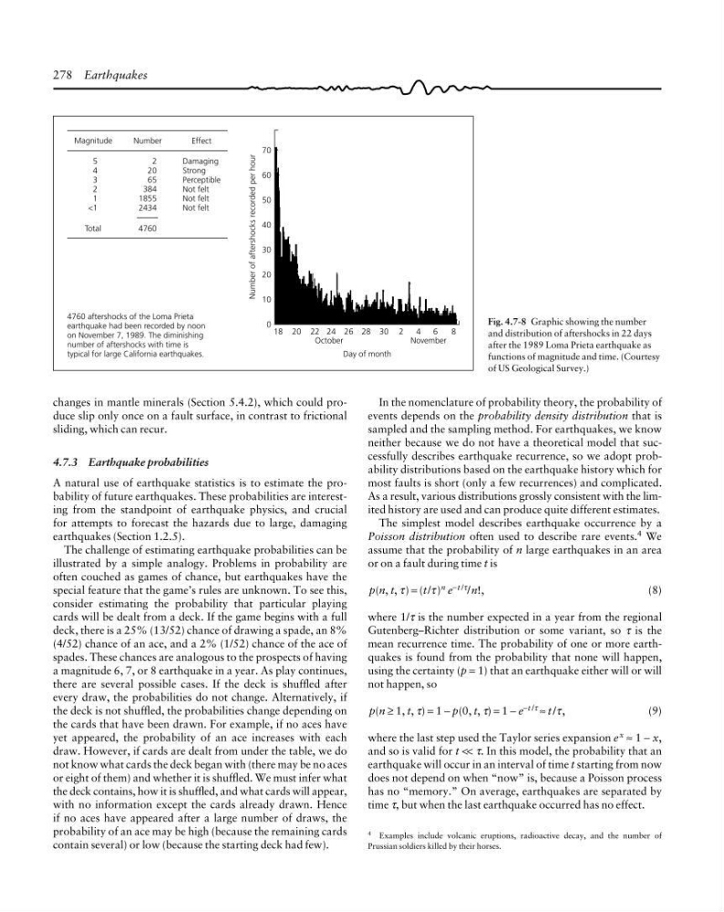
4760 aftershocks of the Loma Prieta
earthquake had been recorded by noon
on November 7, 1989. The diminishing
number of aftershocks with time is
typical for large California earthquakes.
Number of aftershocks recorded per hour
70
60
50
40
30
20
10
0
18 20 22 24 26 28 30 2
4
6
8
October
November
Day of month
2
20
65
384
1855
2434
4760
Fig. 4.7-8 Graphic showing the number
and distribution of aftershocks in 22 days
after the 1989 Loma Prieta earthquake as
functions of magnitude and time. (Courtesy
of US Geological Survey.)
4 Examples include volcanic eruptions, radioactive decay, and the number of
Prussian soldiers killed by their horses.
In the nomenclature of probability theory, the probability of
events depends on the probability density distribution that is
sampled and the sampling method. For earthquakes, we know
neither because we do not have a theoretical model that successfully describes earthquake recurrence, so we adopt probability distributions based on the earthquake history which for
most faults is short (only a few recurrences) and complicated.
As a result, various distributions grossly consistent with the limited history are used and can produce quite different estimates.
The simplest model describes earthquake occurrence by a
Poisson distribution often used to describe rare events. 4 We
assume that the probability of n large earthquakes in an area
or on a fault during time t is
p(n, t, τ) = (t/τ ) n e −t /τ /n!,
(8)
where 1/τ is the number expected in a year from the regional
Gutenberg–Richter distribution or some variant, so τ is the
mean recurrence time. The probability of one or more earthquakes is found from the probability that none will happen,
using the certainty (p = 1) that an earthquake either will or will
not happen, so
p(n ≥ 1, t, τ) = 1 − p(0, t, τ) = 1 − e −t /τ ≈ t /τ ,
(9)
where the last step used the Taylor series expansion e
x
≈ 1 − x,
and so is valid for t << τ. In this model, the probability that an
earthquake will occur in an interval of time t starting from now
does not depend on when “now” is, because a Poisson process
has no “memory.” On average, earthquakes are separated by
time τ, but when the last earthquake occurred has no effect.
changes in mantle minerals (Section 5.4.2), which could produce slip only once on a fault surface, in contrast to frictional
sliding, which can recur.
4.7.3 Earthquake probabilities
A natural use of earthquake statistics is to estimate the probability of future earthquakes. These probabilities are interesting from the standpoint of earthquake physics, and crucial
for attempts to forecast the hazards due to large, damaging
earthquakes (Section 1.2.5).
The challenge of estimating earthquake probabilities can be
illustrated by a simple analogy. Problems in probability are
often couched as games of chance, but earthquakes have the
special feature that the game’s rules are unknown. To see this,
consider estimating the probability that particular playing
cards will be dealt from a deck. If the game begins with a full
deck, there is a 25% (13/52) chance of drawing a spade, an 8%
(4/52) chance of an ace, and a 2% (1/52) chance of the ace of
spades. These chances are analogous to the prospects of having
a magnitude 6, 7, or 8 earthquake in a year. As play continues,
there are several possible cases. If the deck is shuffled after
every draw, the probabilities do not change. Alternatively, if
the deck is not shuffled, the probabilities change depending on
the cards that have been drawn. For example, if no aces have
yet appeared, the probability of an ace increases with each
draw. However, if cards are dealt from under the table, we do
not know what cards the deck began with (there may be no aces
or eight of them) and whether it is shuffled. We must infer what
the deck contains, how it is shuffled, and what cards will appear,
with no information except the cards already drawn. Hence
if no aces have appeared after a large number of draws, the
probability of an ace may be high (because the remaining cards
contain several) or low (because the starting deck had few).
Magnitude
Number
Effect
5
4
3
2
1
<1
Damaging
Strong
Perceptible
Not felt
Not felt
Not felt
Total
4760 aftershocks of the Loma Prieta
earthquake had been recorded by noon
on November 7, 1989. The diminishing
number of aftershocks with time is
typical for large California earthquakes.
Number of aftershocks recorded per hour
70
60
50
40
30
20
10
0
18 20 22 24 26 28 30 2
4
6
8
October
November
Day of month
2
20
65
384
1855
2434
4760
Fig. 4.7-8 Graphic showing the number
and distribution of aftershocks in 22 days
after the 1989 Loma Prieta earthquake as
functions of magnitude and time. (Courtesy
of US Geological Survey.)
4 Examples include volcanic eruptions, radioactive decay, and the number of
Prussian soldiers killed by their horses.
In the nomenclature of probability theory, the probability of
events depends on the probability density distribution that is
sampled and the sampling method. For earthquakes, we know
neither because we do not have a theoretical model that successfully describes earthquake recurrence, so we adopt probability distributions based on the earthquake history which for
most faults is short (only a few recurrences) and complicated.
As a result, various distributions grossly consistent with the limited history are used and can produce quite different estimates.
The simplest model describes earthquake occurrence by a
Poisson distribution often used to describe rare events. 4 We
assume that the probability of n large earthquakes in an area
or on a fault during time t is
p(n, t, τ) = (t/τ ) n e −t /τ /n!,
(8)
where 1/τ is the number expected in a year from the regional
Gutenberg–Richter distribution or some variant, so τ is the
mean recurrence time. The probability of one or more earthquakes is found from the probability that none will happen,
using the certainty (p = 1) that an earthquake either will or will
not happen, so
p(n ≥ 1, t, τ) = 1 − p(0, t, τ) = 1 − e −t /τ ≈ t /τ ,
(9)
where the last step used the Taylor series expansion e
x
≈ 1 − x,
and so is valid for t << τ. In this model, the probability that an
earthquake will occur in an interval of time t starting from now
does not depend on when “now” is, because a Poisson process
has no “memory.” On average, earthquakes are separated by
time τ, but when the last earthquake occurred has no effect.
changes in mantle minerals (Section 5.4.2), which could produce slip only once on a fault surface, in contrast to frictional
sliding, which can recur.
4.7.3 Earthquake probabilities
A natural use of earthquake statistics is to estimate the probability of future earthquakes. These probabilities are interesting from the standpoint of earthquake physics, and crucial
for attempts to forecast the hazards due to large, damaging
earthquakes (Section 1.2.5).
The challenge of estimating earthquake probabilities can be
illustrated by a simple analogy. Problems in probability are
often couched as games of chance, but earthquakes have the
special feature that the game’s rules are unknown. To see this,
consider estimating the probability that particular playing
cards will be dealt from a deck. If the game begins with a full
deck, there is a 25% (13/52) chance of drawing a spade, an 8%
(4/52) chance of an ace, and a 2% (1/52) chance of the ace of
spades. These chances are analogous to the prospects of having
a magnitude 6, 7, or 8 earthquake in a year. As play continues,
there are several possible cases. If the deck is shuffled after
every draw, the probabilities do not change. Alternatively, if
the deck is not shuffled, the probabilities change depending on
the cards that have been drawn. For example, if no aces have
yet appeared, the probability of an ace increases with each
draw. However, if cards are dealt from under the table, we do
not know what cards the deck began with (there may be no aces
or eight of them) and whether it is shuffled. We must infer what
the deck contains, how it is shuffled, and what cards will appear,
with no information except the cards already drawn. Hence
if no aces have appeared after a large number of draws, the
probability of an ace may be high (because the remaining cards
contain several) or low (because the starting deck had few).