

total population. Thus the b value is reasonably well estimated
from the smaller earthquakes, but not the largest ones. This
effect may occur if the number of large earthquakes in the
study is small. For example, we might expect this for individual faults, even in a region whose overall seismicity obeys
a Gutenberg–Richter distribution.
A final point worth noting is that although the Gutenberg–
Richter distribution predicts the frequency of arbitrarily large
earthquakes, such earthquakes may not actually occur. As we
have seen, the area available for faulting limits earthquake size.
For example, we will see in Section 5.3.3 that the maximum
moment of mid-ocean ridge earthquakes varies inversely with
spreading rate. As a result, regional studies often assume the
existence of a maximum magnitude, sometimes based on the
earthquake history, in the Gutenberg–Richter distribution.
This assumption has interesting implications, because on many
plate boundaries the motion inferred from earthquake histories
seems to be significantly less than the plate motion (Sections
5.3.3, 5.4.3, 5.6.2). Hence, either the missing motion occurs in
very large, rare earthquakes, or much of the motion occurs by
aseismic processes. Which of these is the case is also of interest
for seismic hazard studies.
4.7.2 Aftershocks
The smaller aftershocks following a mainshock have a characteristic distribution in size and time. As previously noted (e.g.,
Fig. 4.5-9), most aftershocks occur on or near the mainshock’s
fault plane, so their locations are used to distinguish between
the fault and auxiliary planes and to estimate the fault area.
The largest aftershock is usually more than a magnitude unit
smaller than the mainshock, and the aftershocks have a size
distribution with b near 1, so the total energy released by the
aftershocks is usually less than 10% of that of the mainshock.
Most of the aftershocks occur soon after the mainshock, and
the remainder decay with time in a quasi-hyperbolic manner.
This decay is described by a relation now called Omori’s law, 3
n
C
K t
P
(
)
,
=
+
(7)
where n is the frequency of aftershocks at a time t after the
mainshock, with K, C, and P as fault-dependent constants. P is
typically about 1. This decay is illustrated by the aftershocks of
the 1989 (M s 7.1) Loma Prieta earthquake (Fig. 4.7-8).
The aftershock decay is thought to reflect stress readjustment
following the stress changes due to the main shock. An intriguing exception to Omori’s law is that most deep earthquakes
have many fewer, and often no, detected aftershocks. This difference may reflect deep earthquakes resulting from phase
Cumulative number of earthquakes
2000
1000
300
100
30
10
3
1
3
4
5
6
7
8
Magnitude
L
o
g
1
0
N
c
u
m
=
5
.
3
3
–
0
.
6
7
M
L
o
g
N
su
b
=
4
.
3
3
–
0
.
6
7
M
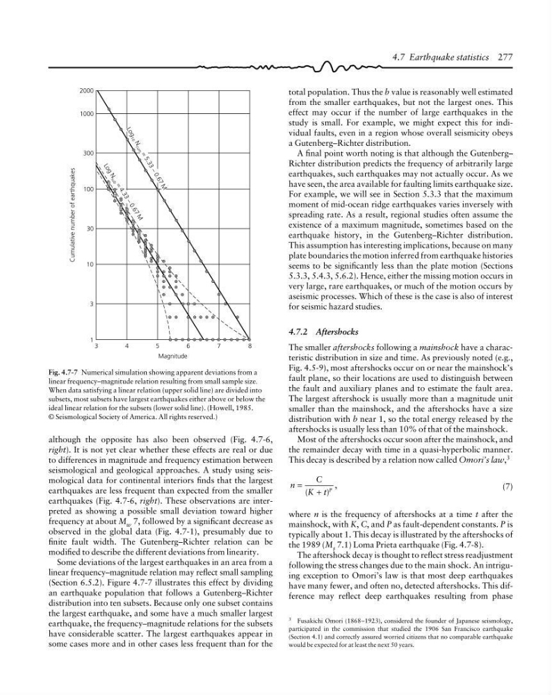
Fig. 4.7-7 Numerical simulation showing apparent deviations from a
linear frequency–magnitude relation resulting from small sample size.
When data satisfying a linear relation (upper solid line) are divided into
subsets, most subsets have largest earthquakes either above or below the
ideal linear relation for the subsets (lower solid line). (Howell, 1985.
© Seismological Society of America. All rights reserved.)
3 Fusakichi Omori (1868–1923), considered the founder of Japanese seismology,
participated in the commission that studied the 1906 San Francisco earthquake
(Section 4.1) and correctly assured worried citizens that no comparable earthquake
would be expected for at least the next 50 years.
4.7 Earthquake statistics 277
although the opposite has also been observed (Fig. 4.7-6,
right). It is not yet clear whether these effects are real or due
to differences in magnitude and frequency estimation between
seismological and geological approaches. A study using seismological data for continental interiors finds that the largest
earthquakes are less frequent than expected from the smaller
earthquakes (Fig. 4.7-6, right). These observations are interpreted as showing a possible small deviation toward higher
frequency at about M w 7, followed by a significant decrease as
observed in the global data (Fig. 4.7-1), presumably due to
finite fault width. The Gutenberg–Richter relation can be
modified to describe the different deviations from linearity.
Some deviations of the largest earthquakes in an area from a
linear frequency–magnitude relation may reflect small sampling
(Section 6.5.2). Figure 4.7-7 illustrates this effect by dividing
an earthquake population that follows a Gutenberg–Richter
distribution into ten subsets. Because only one subset contains
the largest earthquake, and some have a much smaller largest
earthquake, the frequency–magnitude relations for the subsets
have considerable scatter. The largest earthquakes appear in
some cases more and in other cases less frequent than for the
from the smaller earthquakes, but not the largest ones. This
effect may occur if the number of large earthquakes in the
study is small. For example, we might expect this for individual faults, even in a region whose overall seismicity obeys
a Gutenberg–Richter distribution.
A final point worth noting is that although the Gutenberg–
Richter distribution predicts the frequency of arbitrarily large
earthquakes, such earthquakes may not actually occur. As we
have seen, the area available for faulting limits earthquake size.
For example, we will see in Section 5.3.3 that the maximum
moment of mid-ocean ridge earthquakes varies inversely with
spreading rate. As a result, regional studies often assume the
existence of a maximum magnitude, sometimes based on the
earthquake history, in the Gutenberg–Richter distribution.
This assumption has interesting implications, because on many
plate boundaries the motion inferred from earthquake histories
seems to be significantly less than the plate motion (Sections
5.3.3, 5.4.3, 5.6.2). Hence, either the missing motion occurs in
very large, rare earthquakes, or much of the motion occurs by
aseismic processes. Which of these is the case is also of interest
for seismic hazard studies.
4.7.2 Aftershocks
The smaller aftershocks following a mainshock have a characteristic distribution in size and time. As previously noted (e.g.,
Fig. 4.5-9), most aftershocks occur on or near the mainshock’s
fault plane, so their locations are used to distinguish between
the fault and auxiliary planes and to estimate the fault area.
The largest aftershock is usually more than a magnitude unit
smaller than the mainshock, and the aftershocks have a size
distribution with b near 1, so the total energy released by the
aftershocks is usually less than 10% of that of the mainshock.
Most of the aftershocks occur soon after the mainshock, and
the remainder decay with time in a quasi-hyperbolic manner.
This decay is described by a relation now called Omori’s law, 3
n
C
K t
P
(
)
,
=
+
(7)
where n is the frequency of aftershocks at a time t after the
mainshock, with K, C, and P as fault-dependent constants. P is
typically about 1. This decay is illustrated by the aftershocks of
the 1989 (M s 7.1) Loma Prieta earthquake (Fig. 4.7-8).
The aftershock decay is thought to reflect stress readjustment
following the stress changes due to the main shock. An intriguing exception to Omori’s law is that most deep earthquakes
have many fewer, and often no, detected aftershocks. This difference may reflect deep earthquakes resulting from phase
Cumulative number of earthquakes
2000
1000
300
100
30
10
3
1
3
4
5
6
7
8
Magnitude
L
o
g
1
0
N
c
u
m
=
5
.
3
3
–
0
.
6
7
M
L
o
g
N
su
b
=
4
.
3
3
–
0
.
6
7
M
Fig. 4.7-7 Numerical simulation showing apparent deviations from a
linear frequency–magnitude relation resulting from small sample size.
When data satisfying a linear relation (upper solid line) are divided into
subsets, most subsets have largest earthquakes either above or below the
ideal linear relation for the subsets (lower solid line). (Howell, 1985.
© Seismological Society of America. All rights reserved.)
3 Fusakichi Omori (1868–1923), considered the founder of Japanese seismology,
participated in the commission that studied the 1906 San Francisco earthquake
(Section 4.1) and correctly assured worried citizens that no comparable earthquake
would be expected for at least the next 50 years.
4.7 Earthquake statistics 277
although the opposite has also been observed (Fig. 4.7-6,
right). It is not yet clear whether these effects are real or due
to differences in magnitude and frequency estimation between
seismological and geological approaches. A study using seismological data for continental interiors finds that the largest
earthquakes are less frequent than expected from the smaller
earthquakes (Fig. 4.7-6, right). These observations are interpreted as showing a possible small deviation toward higher
frequency at about M w 7, followed by a significant decrease as
observed in the global data (Fig. 4.7-1), presumably due to
finite fault width. The Gutenberg–Richter relation can be
modified to describe the different deviations from linearity.
Some deviations of the largest earthquakes in an area from a
linear frequency–magnitude relation may reflect small sampling
(Section 6.5.2). Figure 4.7-7 illustrates this effect by dividing
an earthquake population that follows a Gutenberg–Richter
distribution into ten subsets. Because only one subset contains
the largest earthquake, and some have a much smaller largest
earthquake, the frequency–magnitude relations for the subsets
have considerable scatter. The largest earthquakes appear in
some cases more and in other cases less frequent than for the