

276 Earthquakes
Depth (km)
Distance along fault (km)
0
5
10
>1
0.8
0.6
NW
1971–1984.3
SE
1984 M 6.2 Morgan Hill
b value
−20
−10
0
10
20
30
40
2000
Cumulative moment (dyn-cm)
8 × 10
29
6 × 10
29
4 × 10
29
2 × 10
29
0
1976
1980
1984
1988
1992
1996
Year
All
earthquakes
M W < 6.5
M W < 7.1
M W < 7.5
M W < 7.9
mon, earthquakes contribute less, so the contribution of earthquakes with magnitudes less than 6 is negligible.
Although b values approximately equal 1 over long time
scales and large spatial scales, significant variations occur on
smaller scales. The b value of earthquake swarms is often much
larger than 1, sometimes approaching 2.5. These swarms,
which lack a mainshock, are often associated with volcanic
regions, and may result from processes such as the migration
of magmatic fluids or caldera development. For example,
seismicity associated with the collapse of the Fernandina
caldera in the Galapagos Islands in 1968 had b ≈ 1.9, indicating
many small earthquakes but fewer large ones than expected.
The b value also varies regionally, both spatially and with
depth. Figure 4.7-5 shows the variation in b value on a segment
of the Calavaras fault in California. Some patches have b values
much less than 1, implying shorter recurrence time. These
patches have been interpreted as possible asperities or stress
concentrations, perhaps reflecting variations in frictional properties along the fault, which may control the recurrence of the
next large earthquake and have large moment release during it.
Other intriguing possible deviations from b = 1 have been
reported. Figure 4.7-6 (left) shows earthquake magnitudes
and frequencies for large earthquakes inferred from geological
paleoseismic studies, which deviate from the seismologically
determined frequency–magnitude data. These observations have
been interpreted as showing large (sometimes termed characteristic) earthquakes more frequent than would be expected
from the linear relation derived from the instrumental data,
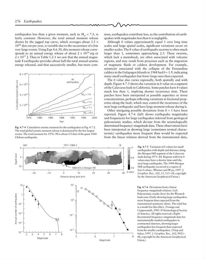
earthquakes less than a given moment, such as M w < 7.5, is
fairly constant. However, the total annual moment release
shown by the jagged top curve, which averages about 3.5 ×
10 28 dyn-cm per year, is variable due to the occurrence of a few
very large events. Using Eqn 4.6.30, this moment release corresponds to an annual energy release of about 2 × 10 24 erg or
2 × 10 17 J. Thus in Table 1.2-1 we saw that the annual magnitude 8 earthquake provides about half the total annual seismic
energy released, and that successively smaller, but more comAnnual number of earthquakes
10
1
10
−1
10
−2
10
−3
10
−4
2
3
4
5
6
7
8
Magnitude
10
−1
5
6
7
8
10
−2
10
0
10
1
Magnitude
Fig. 4.7-6 Deviations from a linear
frequency–magnitude relation. Left:
Paleoseismic results (box) for the Wasatch
fault zone (Utah) showing large earthquakes
more frequent than expected from the
instrumental seismicity (dots). The solid line
is a model for this effect. (Youngs and
Coppersmith, 1985. © Seismological Society
of America. All rights reserved.) Right:
Incremental frequency–magnitude data for
instrumentally studied earthquakes in
continental interiors, showing larger
earthquakes less frequent than expected
from the smaller earthquakes. (Triep and
Sykes, 1997. J. Geophys. Res., 102, 9923–
48, copyright by the American Geophysical
Union.)
Fig. 4.7-5 Variation of b values for small
earthquakes with depth and distance along
the Morgan Hill segment of the Calaveras
fault during 1971–84. Regions with low b
values may have a shorter time until the
next large earthquake. The 1984 Morgan
Hill earthquake occurred in a region of
low b values. (Wiemer and Wyss, 1997. J.
Geophys. Res., 102, 15, 115–28, copyright
by the American Geophysical Union.)
Fig. 4.7-4 Cumulative seismic moment for the earthquakes in Fig. 4.7-2.
The total global seismic moment release is dominated by the few largest
events. The total moment for 1976–98 is about 1/3 that of the giant 1960
Chilean earthquake.
Depth (km)
Distance along fault (km)
0
5
10
>1
0.8
0.6
NW
1971–1984.3
SE
1984 M 6.2 Morgan Hill
b value
−20
−10
0
10
20
30
40
2000
Cumulative moment (dyn-cm)
8 × 10
29
6 × 10
29
4 × 10
29
2 × 10
29
0
1976
1980
1984
1988
1992
1996
Year
All
earthquakes
M W < 6.5
M W < 7.1
M W < 7.5
M W < 7.9
mon, earthquakes contribute less, so the contribution of earthquakes with magnitudes less than 6 is negligible.
Although b values approximately equal 1 over long time
scales and large spatial scales, significant variations occur on
smaller scales. The b value of earthquake swarms is often much
larger than 1, sometimes approaching 2.5. These swarms,
which lack a mainshock, are often associated with volcanic
regions, and may result from processes such as the migration
of magmatic fluids or caldera development. For example,
seismicity associated with the collapse of the Fernandina
caldera in the Galapagos Islands in 1968 had b ≈ 1.9, indicating
many small earthquakes but fewer large ones than expected.
The b value also varies regionally, both spatially and with
depth. Figure 4.7-5 shows the variation in b value on a segment
of the Calavaras fault in California. Some patches have b values
much less than 1, implying shorter recurrence time. These
patches have been interpreted as possible asperities or stress
concentrations, perhaps reflecting variations in frictional properties along the fault, which may control the recurrence of the
next large earthquake and have large moment release during it.
Other intriguing possible deviations from b = 1 have been
reported. Figure 4.7-6 (left) shows earthquake magnitudes
and frequencies for large earthquakes inferred from geological
paleoseismic studies, which deviate from the seismologically
determined frequency–magnitude data. These observations have
been interpreted as showing large (sometimes termed characteristic) earthquakes more frequent than would be expected
from the linear relation derived from the instrumental data,
earthquakes less than a given moment, such as M w < 7.5, is
fairly constant. However, the total annual moment release
shown by the jagged top curve, which averages about 3.5 ×
10 28 dyn-cm per year, is variable due to the occurrence of a few
very large events. Using Eqn 4.6.30, this moment release corresponds to an annual energy release of about 2 × 10 24 erg or
2 × 10 17 J. Thus in Table 1.2-1 we saw that the annual magnitude 8 earthquake provides about half the total annual seismic
energy released, and that successively smaller, but more comAnnual number of earthquakes
10
1
10
−1
10
−2
10
−3
10
−4
2
3
4
5
6
7
8
Magnitude
10
−1
5
6
7
8
10
−2
10
0
10
1
Magnitude
Fig. 4.7-6 Deviations from a linear
frequency–magnitude relation. Left:
Paleoseismic results (box) for the Wasatch
fault zone (Utah) showing large earthquakes
more frequent than expected from the
instrumental seismicity (dots). The solid line
is a model for this effect. (Youngs and
Coppersmith, 1985. © Seismological Society
of America. All rights reserved.) Right:
Incremental frequency–magnitude data for
instrumentally studied earthquakes in
continental interiors, showing larger
earthquakes less frequent than expected
from the smaller earthquakes. (Triep and
Sykes, 1997. J. Geophys. Res., 102, 9923–
48, copyright by the American Geophysical
Union.)
Fig. 4.7-5 Variation of b values for small
earthquakes with depth and distance along
the Morgan Hill segment of the Calaveras
fault during 1971–84. Regions with low b
values may have a shorter time until the
next large earthquake. The 1984 Morgan
Hill earthquake occurred in a region of
low b values. (Wiemer and Wyss, 1997. J.
Geophys. Res., 102, 15, 115–28, copyright
by the American Geophysical Union.)
Fig. 4.7-4 Cumulative seismic moment for the earthquakes in Fig. 4.7-2.
The total global seismic moment release is dominated by the few largest
events. The total moment for 1976–98 is about 1/3 that of the giant 1960
Chilean earthquake.