

Length (km)
1000
100
10
1
24
25
26
27
28
29
30
31
interplate
Japan intraplate
western USA
strike-slip
Log M 0 (dyn-cm)
A model for this phenomenon based on the concept of scale
invariance assumes that the probability of an earthquake of
a given size on a fault is inversely proportional to the area of
faulting involved, so the number N of earthquakes with fault
area greater than S should obey a frequency–area relation like
those for magnitude or moment
log N = c − log S.
(5)
We saw in Eqn 4.6.17 that for constant stress drop the
moment is proportional to S
3/2
, or the fault dimension L cubed,
so we expect
log N = c − 2/3 log M 0 ,
(6)
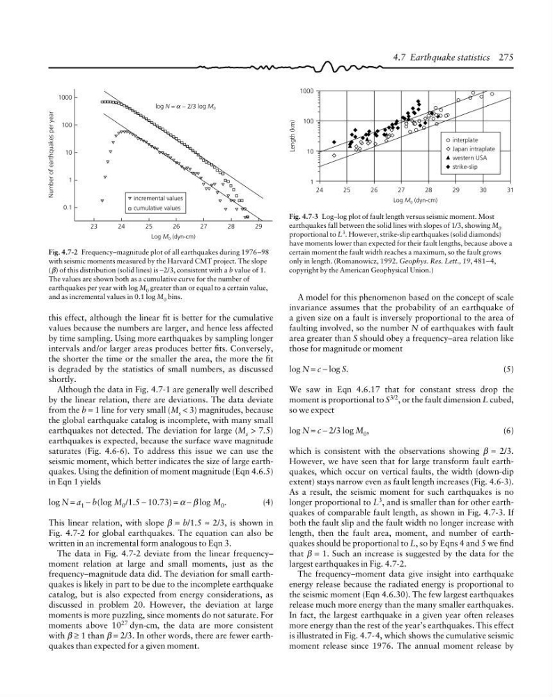
which is consistent with the observations showing β ≈ 2/3.
However, we have seen that for large transform fault earthquakes, which occur on vertical faults, the width (down-dip
extent) stays narrow even as fault length increases (Fig. 4.6-3).
As a result, the seismic moment for such earthquakes is no
longer proportional to L 3 , and is smaller than for other earthquakes of comparable fault length, as shown in Fig. 4.7-3. If
both the fault slip and the fault width no longer increase with
length, then the fault area, moment, and number of earthquakes should be proportional to L, so by Eqns 4 and 5 we find
that β = 1. Such an increase is suggested by the data for the
largest earthquakes in Fig. 4.7-2.
The frequency–moment data give insight into earthquake
energy release because the radiated energy is proportional to
the seismic moment (Eqn 4.6.30). The few largest earthquakes
release much more energy than the many smaller earthquakes.
In fact, the largest earthquake in a given year often releases
more energy than the rest of the year’s earthquakes. This effect
is illustrated in Fig. 4.7-4, which shows the cumulative seismic
moment release since 1976. The annual moment release by
Fig. 4.7-2 Frequency–magnitude plot of all earthquakes during 1976–98
with seismic moments measured by the Harvard CMT project. The slope
(β) of this distribution (solid lines) is −2/3, consistent with a b value of 1.
The values are shown both as a cumulative curve for the number of
earthquakes per year with log M 0 greater than or equal to a certain value,
and as incremental values in 0.1 log M 0 bins.
Number of earthquakes per year
1000
100
10
1
0.1
log N = α − 2/3 log M 0
incremental values
cumulative values
23
26
27
28
Log M 0 (dyn-cm)
α
24
25
29
this effect, although the linear fit is better for the cumulative
values because the numbers are larger, and hence less affected
by time sampling. Using more earthquakes by sampling longer
intervals and/or larger areas produces better fits. Conversely,
the shorter the time or the smaller the area, the more the fit
is degraded by the statistics of small numbers, as discussed
shortly.
Although the data in Fig. 4.7-1 are generally well described
by the linear relation, there are deviations. The data deviate
from the b = 1 line for very small (M s < 3) magnitudes, because
the global earthquake catalog is incomplete, with many small
earthquakes not detected. The deviation for large (M s > 7.5)
earthquakes is expected, because the surface wave magnitude
saturates (Fig. 4.6-6). To address this issue we can use the
seismic moment, which better indicates the size of large earthquakes. Using the definition of moment magnitude (Eqn 4.6.5)
in Eqn 1 yields
log N = a 1 − b(log M 0 /1.5 − 10.73) = α − β log M 0 .
(4)
This linear relation, with slope β = b/1.5 ≈ 2/3, is shown in
Fig. 4.7-2 for global earthquakes. The equation can also be
written in an incremental form analogous to Eqn 3.
The data in Fig. 4.7-2 deviate from the linear frequency–
moment relation at large and small moments, just as the
frequency–magnitude data did. The deviation for small earthquakes is likely in part to be due to the incomplete earthquake
catalog, but is also expected from energy considerations, as
discussed in problem 20. However, the deviation at large
moments is more puzzling, since moments do not saturate. For
moments above 10 27 dyn-cm, the data are more consistent
with β ≥ 1 than β = 2/3. In other words, there are fewer earthquakes than expected for a given moment.
Fig. 4.7-3 Log–log plot of fault length versus seismic moment. Most
earthquakes fall between the solid lines with slopes of 1/3, showing M 0
proportional to L
3 . However, strike-slip earthquakes (solid diamonds)
have moments lower than expected for their fault lengths, because above a
certain moment the fault width reaches a maximum, so the fault grows
only in length. (Romanowicz, 1992. Geophys. Res. Lett., 19, 481–4,
copyright by the American Geophysical Union.)
4.7 Earthquake statistics 275
1000
100
10
1
24
25
26
27
28
29
30
31
interplate
Japan intraplate
western USA
strike-slip
Log M 0 (dyn-cm)
A model for this phenomenon based on the concept of scale
invariance assumes that the probability of an earthquake of
a given size on a fault is inversely proportional to the area of
faulting involved, so the number N of earthquakes with fault
area greater than S should obey a frequency–area relation like
those for magnitude or moment
log N = c − log S.
(5)
We saw in Eqn 4.6.17 that for constant stress drop the
moment is proportional to S
3/2
, or the fault dimension L cubed,
so we expect
log N = c − 2/3 log M 0 ,
(6)
which is consistent with the observations showing β ≈ 2/3.
However, we have seen that for large transform fault earthquakes, which occur on vertical faults, the width (down-dip
extent) stays narrow even as fault length increases (Fig. 4.6-3).
As a result, the seismic moment for such earthquakes is no
longer proportional to L 3 , and is smaller than for other earthquakes of comparable fault length, as shown in Fig. 4.7-3. If
both the fault slip and the fault width no longer increase with
length, then the fault area, moment, and number of earthquakes should be proportional to L, so by Eqns 4 and 5 we find
that β = 1. Such an increase is suggested by the data for the
largest earthquakes in Fig. 4.7-2.
The frequency–moment data give insight into earthquake
energy release because the radiated energy is proportional to
the seismic moment (Eqn 4.6.30). The few largest earthquakes
release much more energy than the many smaller earthquakes.
In fact, the largest earthquake in a given year often releases
more energy than the rest of the year’s earthquakes. This effect
is illustrated in Fig. 4.7-4, which shows the cumulative seismic
moment release since 1976. The annual moment release by
Fig. 4.7-2 Frequency–magnitude plot of all earthquakes during 1976–98
with seismic moments measured by the Harvard CMT project. The slope
(β) of this distribution (solid lines) is −2/3, consistent with a b value of 1.
The values are shown both as a cumulative curve for the number of
earthquakes per year with log M 0 greater than or equal to a certain value,
and as incremental values in 0.1 log M 0 bins.
Number of earthquakes per year
1000
100
10
1
0.1
log N = α − 2/3 log M 0
incremental values
cumulative values
23
26
27
28
Log M 0 (dyn-cm)
α
24
25
29
this effect, although the linear fit is better for the cumulative
values because the numbers are larger, and hence less affected
by time sampling. Using more earthquakes by sampling longer
intervals and/or larger areas produces better fits. Conversely,
the shorter the time or the smaller the area, the more the fit
is degraded by the statistics of small numbers, as discussed
shortly.
Although the data in Fig. 4.7-1 are generally well described
by the linear relation, there are deviations. The data deviate
from the b = 1 line for very small (M s < 3) magnitudes, because
the global earthquake catalog is incomplete, with many small
earthquakes not detected. The deviation for large (M s > 7.5)
earthquakes is expected, because the surface wave magnitude
saturates (Fig. 4.6-6). To address this issue we can use the
seismic moment, which better indicates the size of large earthquakes. Using the definition of moment magnitude (Eqn 4.6.5)
in Eqn 1 yields
log N = a 1 − b(log M 0 /1.5 − 10.73) = α − β log M 0 .
(4)
This linear relation, with slope β = b/1.5 ≈ 2/3, is shown in
Fig. 4.7-2 for global earthquakes. The equation can also be
written in an incremental form analogous to Eqn 3.
The data in Fig. 4.7-2 deviate from the linear frequency–
moment relation at large and small moments, just as the
frequency–magnitude data did. The deviation for small earthquakes is likely in part to be due to the incomplete earthquake
catalog, but is also expected from energy considerations, as
discussed in problem 20. However, the deviation at large
moments is more puzzling, since moments do not saturate. For
moments above 10 27 dyn-cm, the data are more consistent
with β ≥ 1 than β = 2/3. In other words, there are fewer earthquakes than expected for a given moment.
Fig. 4.7-3 Log–log plot of fault length versus seismic moment. Most
earthquakes fall between the solid lines with slopes of 1/3, showing M 0
proportional to L
3 . However, strike-slip earthquakes (solid diamonds)
have moments lower than expected for their fault lengths, because above a
certain moment the fault width reaches a maximum, so the fault grows
only in length. (Romanowicz, 1992. Geophys. Res. Lett., 19, 481–4,
copyright by the American Geophysical Union.)
4.7 Earthquake statistics 275