

274 Earthquakes
4.7 Earthquake statistics
In discussing earthquake source parameters, we saw that interesting insights into earthquake processes, such as magnitude
saturation and constant stress drop, came from considering
general properties of large numbers of earthquakes. Hence
we now turn to some ideas about the statistics of earthquake
populations, which have implications for both source processes and hazard estimation. 1
4.7.1 Frequency –magnitude relations
As mentioned in Section 1.2, the number of earthquakes
that occur yearly around the world varies with magnitude, with
successively smaller earthquakes being more common. This
observation was quantified by Gutenberg and Richter 2 in the
1940s via the logarithmic earthquake frequency–magnitude
relation
log N = a 1 − bM,
(1)
in which N is the number of earthquakes with magnitude greater
than or equal to M occurring in a given time. The distribution is
described by a linear relation, with constants a 1 and b. It turns
out that although the intercept, a 1 , depends on the number of
earthquakes in the time and region sampled, the slope, b, is
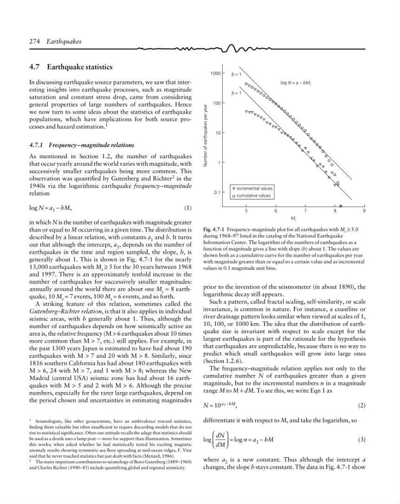
generally about 1. This is shown in Fig. 4.7-1 for the nearly
13,000 earthquakes with M s ≥ 5 for the 30 years between 1968
and 1997. There is an approximately tenfold increase in the
number of earthquakes for successively smaller magnitudes:
annually around the world there are about one M s = 8 earthquake, 10 M s = 7 events, 100 M s = 6 events, and so forth.
A striking feature of this relation, sometimes called the
Gutenberg–Richter relation, is that it also applies in individual
seismic areas, with b generally about 1. Thus, although the
number of earthquakes depends on how seismically active an
area is, the relative frequency (M > 6 earthquakes about 10 times
more common than M > 7, etc.) still applies. For example, in
the past 1300 years Japan is estimated to have had about 190
earthquakes with M > 7 and 20 with M > 8. Similarly, since
1816 southern California has had about 180 earthquakes with
M > 6, 24 with M > 7, and 1 with M > 8; whereas the New
Madrid (central USA) seismic zone has had about 16 earthquakes with M > 5 and 2 with M > 6. Although the precise
numbers, especially for the rarer large earthquakes, depend on
the period chosen and uncertainties in estimating magnitudes
Fig. 4.7-1 Frequency–magnitude plot for all earthquakes with M s ≥ 5.0
during 1968–97 listed in the catalog of the National Earthquake
Information Center. The logarithm of the numbers of earthquakes as a
function of magnitude gives a line with slope (b) about 1. The values are
shown both as a cumulative curve for the number of earthquakes per year
with magnitude greater than or equal to a certain value and as incremental
values in 0.1 magnitude unit bins.
Number of earthquakes per year
1000
100
10
1
0.1
log N = a − bM s
b = 1
b = 1
5
6
7
8
9
M s
incremental values
cumulative values
1 Seismologists, like other geoscientists, have an ambivalence toward statistics,
finding them valuable but often insufficient to require discarding models that do not
rise to statistical significance. Often our attitude recalls the adage that statistics should
be used as a drunk uses a lamp post — more for support than illumination. Sometimes
this works; when asked whether he had statistically tested his exciting magnetic
anomaly results showing symmetric sea floor spreading at mid-ocean ridges, F. Vine
said that he never touched statistics but just dealt with facts (Menard, 1986).
2 The many important contributions to seismology of Beno Gutenberg (1889–1960)
and Charles Richter (1900–85) include quantifying global and regional seismicity.
prior to the invention of the seismometer (in about 1890), the
logarithmic decay still appears.
Such a pattern, called fractal scaling, self-similarity, or scale
invariance, is common in nature. For instance, a coastline or
river drainage pattern looks similar when viewed at scales of 1,
10, 100, or 1000 km. The idea that the distribution of earthquake size is invariant with respect to scale except for the
largest earthquakes is part of the rationale for the hypothesis
that earthquakes are unpredictable, because there is no way to
predict which small earthquakes will grow into large ones
(Section 1.2.6).
The frequency–magnitude relation applies not only to the
cumulative number N of earthquakes greater than a given
magnitude, but to the incremental numbers n in a magnitude
range M to M + dM. To see this, we write Eqn 1 as
N = 10 a1− bM ,
(2)
differentiate it with respect to M, and take the logarithm, so
log
dN
dM
⎛
⎝
⎜
⎞
⎠
⎟ = log n = a 2 − bM
(3)
where a 2 is a new constant. Thus although the intercept a
changes, the slope b stays constant. The data in Fig. 4.7-1 show
4.7 Earthquake statistics
In discussing earthquake source parameters, we saw that interesting insights into earthquake processes, such as magnitude
saturation and constant stress drop, came from considering
general properties of large numbers of earthquakes. Hence
we now turn to some ideas about the statistics of earthquake
populations, which have implications for both source processes and hazard estimation. 1
4.7.1 Frequency –magnitude relations
As mentioned in Section 1.2, the number of earthquakes
that occur yearly around the world varies with magnitude, with
successively smaller earthquakes being more common. This
observation was quantified by Gutenberg and Richter 2 in the
1940s via the logarithmic earthquake frequency–magnitude
relation
log N = a 1 − bM,
(1)
in which N is the number of earthquakes with magnitude greater
than or equal to M occurring in a given time. The distribution is
described by a linear relation, with constants a 1 and b. It turns
out that although the intercept, a 1 , depends on the number of
earthquakes in the time and region sampled, the slope, b, is
generally about 1. This is shown in Fig. 4.7-1 for the nearly
13,000 earthquakes with M s ≥ 5 for the 30 years between 1968
and 1997. There is an approximately tenfold increase in the
number of earthquakes for successively smaller magnitudes:
annually around the world there are about one M s = 8 earthquake, 10 M s = 7 events, 100 M s = 6 events, and so forth.
A striking feature of this relation, sometimes called the
Gutenberg–Richter relation, is that it also applies in individual
seismic areas, with b generally about 1. Thus, although the
number of earthquakes depends on how seismically active an
area is, the relative frequency (M > 6 earthquakes about 10 times
more common than M > 7, etc.) still applies. For example, in
the past 1300 years Japan is estimated to have had about 190
earthquakes with M > 7 and 20 with M > 8. Similarly, since
1816 southern California has had about 180 earthquakes with
M > 6, 24 with M > 7, and 1 with M > 8; whereas the New
Madrid (central USA) seismic zone has had about 16 earthquakes with M > 5 and 2 with M > 6. Although the precise
numbers, especially for the rarer large earthquakes, depend on
the period chosen and uncertainties in estimating magnitudes
Fig. 4.7-1 Frequency–magnitude plot for all earthquakes with M s ≥ 5.0
during 1968–97 listed in the catalog of the National Earthquake
Information Center. The logarithm of the numbers of earthquakes as a
function of magnitude gives a line with slope (b) about 1. The values are
shown both as a cumulative curve for the number of earthquakes per year
with magnitude greater than or equal to a certain value and as incremental
values in 0.1 magnitude unit bins.
Number of earthquakes per year
1000
100
10
1
0.1
log N = a − bM s
b = 1
b = 1
5
6
7
8
9
M s
incremental values
cumulative values
1 Seismologists, like other geoscientists, have an ambivalence toward statistics,
finding them valuable but often insufficient to require discarding models that do not
rise to statistical significance. Often our attitude recalls the adage that statistics should
be used as a drunk uses a lamp post — more for support than illumination. Sometimes
this works; when asked whether he had statistically tested his exciting magnetic
anomaly results showing symmetric sea floor spreading at mid-ocean ridges, F. Vine
said that he never touched statistics but just dealt with facts (Menard, 1986).
2 The many important contributions to seismology of Beno Gutenberg (1889–1960)
and Charles Richter (1900–85) include quantifying global and regional seismicity.
prior to the invention of the seismometer (in about 1890), the
logarithmic decay still appears.
Such a pattern, called fractal scaling, self-similarity, or scale
invariance, is common in nature. For instance, a coastline or
river drainage pattern looks similar when viewed at scales of 1,
10, 100, or 1000 km. The idea that the distribution of earthquake size is invariant with respect to scale except for the
largest earthquakes is part of the rationale for the hypothesis
that earthquakes are unpredictable, because there is no way to
predict which small earthquakes will grow into large ones
(Section 1.2.6).
The frequency–magnitude relation applies not only to the
cumulative number N of earthquakes greater than a given
magnitude, but to the incremental numbers n in a magnitude
range M to M + dM. To see this, we write Eqn 1 as
N = 10 a1− bM ,
(2)
differentiate it with respect to M, and take the logarithm, so
log
dN
dM
⎛
⎝
⎜
⎞
⎠
⎟ = log n = a 2 − bM
(3)
where a 2 is a new constant. Thus although the intercept a
changes, the slope b stays constant. The data in Fig. 4.7-1 show