

Log S (km
2
)
6
5
4
3
interplate
intraplate
1
2
25
26
27
28
29
30
1 0 0 0
1 0 0
1 0
∆
= 1 b a r
σ
Log M 0 (dyn-cm)
Synthetic
30 s
5 s
Source time
function
Stress drop
(bars)
4698
587
174
73
22
Fig. 4.6-10 Synthetic seismograms for different source time functions and
corresponding inferred stress drops. A small uncertainty in source time
function duration results in a large uncertainty in stress drop. (Stein and
Kroeger, 1980. Reproduced with the permission of the American Society
of Mechanical Engineers.)
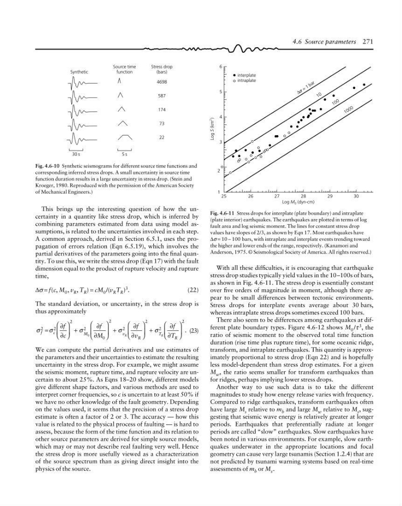
Fig. 4.6-11 Stress drops for interplate (plate boundary) and intraplate
(plate interior) earthquakes. The earthquakes are plotted in terms of log
fault area and log seismic moment. The lines for constant stress drop
values have slopes of 2/3, as shown by Eqn 17. Most earthquakes have
∆σ = 10 – 100 bars, with intraplate and interplate events trending toward
the higher and lower ends of the range, respectively. (Kanamori and
Anderson, 1975. © Seismological Society of America. All rights reserved.)
4.6 Source parameters 271
This brings up the interesting question of how the uncertainty in a quantity like stress drop, which is inferred by
combining parameters estimated from data using model assumptions, is related to the uncertainties involved in each step.
A common approach, derived in Section 6.5.1, uses the propagation of errors relation (Eqn 6.5.19), which involves the
partial derivatives of the parameters going into the final quantity. To use this, we write the stress drop (Eqn 17) with the fault
dimension equal to the product of rupture velocity and rupture
time,
∆σ = f(c, M 0 , v R , T R ) = cM 0 /(v R T R ) 3 .
(22)
The standard deviation, or uncertainty, in the stress drop is
thus approximately
σ σ
σ
σ
σ
f
c
M
v
R
T
R
f
c
f
M
f
v
f
T
R
R
2
2
2
2
0
2
2
2
2
2
0
=
⎛
⎝
⎜
⎞
⎠
⎟ +
⎛
⎝
⎜
⎞
⎠
⎟ +
⎛
⎝
⎜
⎞
⎠
⎟ +
⎛
⎝
⎜
⎞
⎠
⎟
∂
∂
∂
∂
∂
∂
∂
∂
.(23)
We can compute the partial derivatives and use estimates of
the parameters and their uncertainties to estimate the resulting
uncertainty in the stress drop. For example, we might assume
the seismic moment, rupture time, and rupture velocity are uncertain to about 25%. As Eqns 18–20 show, different models
give different shape factors, and various methods are used to
interpret corner frequencies, so c is uncertain to at least 50% if
we have no other knowledge of the fault geometry. Depending
on the values used, it seems that the precision of a stress drop
estimate is often a factor of 2 or 3. The accuracy — how this
value is related to the physical process of faulting — is hard to
assess, because the form of the time function and its relation to
other source parameters are derived for simple source models,
which may or may not describe real faulting very well. Hence
the stress drop is more usefully viewed as a characterization
of the source spectrum than as giving direct insight into the
physics of the source.
With all these difficulties, it is encouraging that earthquake
stress drop studies typically yield values in the 10–100s of bars,
as shown in Fig. 4.6-11. The stress drop is essentially constant
over five orders of magnitude in moment, although there appear to be small differences between tectonic environments.
Stress drops for interplate events average about 30 bars,
whereas intraplate stress drops sometimes exceed 100 bars.
There also seem to be differences among earthquakes at different plate boundary types. Figure 4.6-12 shows M 0 /τ 3 , the
ratio of seismic moment to the observed total time function
duration (rise time plus rupture time), for some oceanic ridge,
transform, and intraplate earthquakes. This quantity is approximately proportional to stress drop (Eqn 22) and is hopefully
less model-dependent than stress drop estimates. For a given
M w , the ratio seems smaller for transform earthquakes than
for ridges, perhaps implying lower stress drops.
Another way to use such data is to take the different
magnitudes to study how energy release varies with frequency.
Compared to ridge earthquakes, transform earthquakes often
have large M s relative to m b and large M w relative to M s , suggesting that seismic wave energy is relatively greater at longer
periods. Earthquakes that preferentially radiate at longer
periods are called “slow” earthquakes. Slow earthquakes have
been noted in various environments. For example, slow earthquakes underwater in the appropriate locations and focal
geometry can cause very large tsunamis (Section 1.2.4) that are
not predicted by tsunami warning systems based on real-time
assessments of m b or M s .
2
)
6
5
4
3
interplate
intraplate
1
2
25
26
27
28
29
30
1 0 0 0
1 0 0
1 0
∆
= 1 b a r
σ
Log M 0 (dyn-cm)
Synthetic
30 s
5 s
Source time
function
Stress drop
(bars)
4698
587
174
73
22
Fig. 4.6-10 Synthetic seismograms for different source time functions and
corresponding inferred stress drops. A small uncertainty in source time
function duration results in a large uncertainty in stress drop. (Stein and
Kroeger, 1980. Reproduced with the permission of the American Society
of Mechanical Engineers.)
Fig. 4.6-11 Stress drops for interplate (plate boundary) and intraplate
(plate interior) earthquakes. The earthquakes are plotted in terms of log
fault area and log seismic moment. The lines for constant stress drop
values have slopes of 2/3, as shown by Eqn 17. Most earthquakes have
∆σ = 10 – 100 bars, with intraplate and interplate events trending toward
the higher and lower ends of the range, respectively. (Kanamori and
Anderson, 1975. © Seismological Society of America. All rights reserved.)
4.6 Source parameters 271
This brings up the interesting question of how the uncertainty in a quantity like stress drop, which is inferred by
combining parameters estimated from data using model assumptions, is related to the uncertainties involved in each step.
A common approach, derived in Section 6.5.1, uses the propagation of errors relation (Eqn 6.5.19), which involves the
partial derivatives of the parameters going into the final quantity. To use this, we write the stress drop (Eqn 17) with the fault
dimension equal to the product of rupture velocity and rupture
time,
∆σ = f(c, M 0 , v R , T R ) = cM 0 /(v R T R ) 3 .
(22)
The standard deviation, or uncertainty, in the stress drop is
thus approximately
σ σ
σ
σ
σ
f
c
M
v
R
T
R
f
c
f
M
f
v
f
T
R
R
2
2
2
2
0
2
2
2
2
2
0
=
⎛
⎝
⎜
⎞
⎠
⎟ +
⎛
⎝
⎜
⎞
⎠
⎟ +
⎛
⎝
⎜
⎞
⎠
⎟ +
⎛
⎝
⎜
⎞
⎠
⎟
∂
∂
∂
∂
∂
∂
∂
∂
.(23)
We can compute the partial derivatives and use estimates of
the parameters and their uncertainties to estimate the resulting
uncertainty in the stress drop. For example, we might assume
the seismic moment, rupture time, and rupture velocity are uncertain to about 25%. As Eqns 18–20 show, different models
give different shape factors, and various methods are used to
interpret corner frequencies, so c is uncertain to at least 50% if
we have no other knowledge of the fault geometry. Depending
on the values used, it seems that the precision of a stress drop
estimate is often a factor of 2 or 3. The accuracy — how this
value is related to the physical process of faulting — is hard to
assess, because the form of the time function and its relation to
other source parameters are derived for simple source models,
which may or may not describe real faulting very well. Hence
the stress drop is more usefully viewed as a characterization
of the source spectrum than as giving direct insight into the
physics of the source.
With all these difficulties, it is encouraging that earthquake
stress drop studies typically yield values in the 10–100s of bars,
as shown in Fig. 4.6-11. The stress drop is essentially constant
over five orders of magnitude in moment, although there appear to be small differences between tectonic environments.
Stress drops for interplate events average about 30 bars,
whereas intraplate stress drops sometimes exceed 100 bars.
There also seem to be differences among earthquakes at different plate boundary types. Figure 4.6-12 shows M 0 /τ 3 , the
ratio of seismic moment to the observed total time function
duration (rise time plus rupture time), for some oceanic ridge,
transform, and intraplate earthquakes. This quantity is approximately proportional to stress drop (Eqn 22) and is hopefully
less model-dependent than stress drop estimates. For a given
M w , the ratio seems smaller for transform earthquakes than
for ridges, perhaps implying lower stress drops.
Another way to use such data is to take the different
magnitudes to study how energy release varies with frequency.
Compared to ridge earthquakes, transform earthquakes often
have large M s relative to m b and large M w relative to M s , suggesting that seismic wave energy is relatively greater at longer
periods. Earthquakes that preferentially radiate at longer
periods are called “slow” earthquakes. Slow earthquakes have
been noted in various environments. For example, slow earthquakes underwater in the appropriate locations and focal
geometry can cause very large tsunamis (Section 1.2.4) that are
not predicted by tsunami warning systems based on real-time
assessments of m b or M s .