

270 Earthquakes
Moment density (dyn-cm)
27
26
25
24
23
0.001
0.010
0.100
1.000
Log frequency (Hz)
–3
Log amplitude (cm-s)
2
1
0
–1
–2
–2
–1
0
1
Log frequency (Hz)
P waves
COL
KIP
TRN
LPB
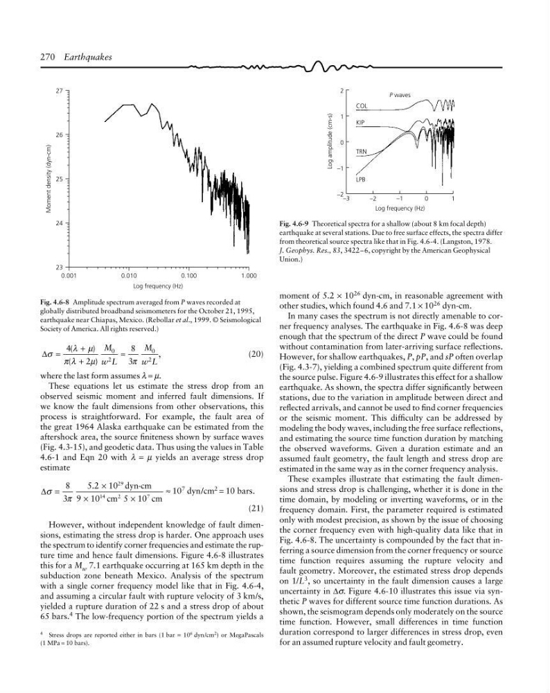
Fig. 4.6-8 Amplitude spectrum averaged from P waves recorded at
globally distributed broadband seismometers for the October 21, 1995,
earthquake near Chiapas, Mexico. (Rebollar et al., 1999. © Seismological
Society of America. All rights reserved.)
4 Stress drops are reported either in bars (1 bar = 10
6 dyn/cm
2
) or MegaPascals
(1 MPa = 10 bars).
Fig. 4.6-9 Theoretical spectra for a shallow (about 8 km focal depth)
earthquake at several stations. Due to free surface effects, the spectra differ
from theoretical source spectra like that in Fig. 4.6-4. (Langston, 1978.
J. Geophys. Res., 83, 3422–6, copyright by the American Geophysical
Union.)
∆σ
λ µ
π λ
µ
π
(
)
(
)
,
=
+
+
≈
4
2
8
3
0
2
0
2
M
w L
M
w L
(20)
where the last form assumes λ = µ.
These equations let us estimate the stress drop from an
observed seismic moment and inferred fault dimensions. If
we know the fault dimensions from other observations, this
process is straightforward. For example, the fault area of
the great 1964 Alaska earthquake can be estimated from the
aftershock area, the source finiteness shown by surface waves
(Fig. 4.3-15), and geodetic data. Thus using the values in Table
4.6-1 and Eqn 20 with λ = µ yields an average stress drop
estimate
∆σ
π
.
=
×
×
×
8
3
5 2 10
9 10
5 10
29
14
2
7
dyn-cm
cm
cm
≈ 10 7 dyn/cm 2 = 10 bars.
(21)
However, without independent knowledge of fault dimensions, estimating the stress drop is harder. One approach uses
the spectrum to identify corner frequencies and estimate the rupture time and hence fault dimensions. Figure 4.6-8 illustrates
this for a M w 7.1 earthquake occurring at 165 km depth in the
subduction zone beneath Mexico. Analysis of the spectrum
with a single corner frequency model like that in Fig. 4.6-4,
and assuming a circular fault with rupture velocity of 3 km/s,
yielded a rupture duration of 22 s and a stress drop of about
65 bars. 4 The low-frequency portion of the spectrum yields a
moment of 5.2 × 10
26 dyn-cm, in reasonable agreement with
other studies, which found 4.6 and 7.1 × 10 26 dyn-cm.
In many cases the spectrum is not directly amenable to corner frequency analyses. The earthquake in Fig. 4.6-8 was deep
enough that the spectrum of the direct P wave could be found
without contamination from later-arriving surface reflections.
However, for shallow earthquakes, P, pP, and sP often overlap
(Fig. 4.3-7), yielding a combined spectrum quite different from
the source pulse. Figure 4.6-9 illustrates this effect for a shallow
earthquake. As shown, the spectra differ significantly between
stations, due to the variation in amplitude between direct and
reflected arrivals, and cannot be used to find corner frequencies
or the seismic moment. This difficulty can be addressed by
modeling the body waves, including the free surface reflections,
and estimating the source time function duration by matching
the observed waveforms. Given a duration estimate and an
assumed fault geometry, the fault length and stress drop are
estimated in the same way as in the corner frequency analysis.
These examples illustrate that estimating the fault dimensions and stress drop is challenging, whether it is done in the
time domain, by modeling or inverting waveforms, or in the
frequency domain. First, the parameter required is estimated
only with modest precision, as shown by the issue of choosing
the corner frequency even with high-quality data like that in
Fig. 4.6-8. The uncertainty is compounded by the fact that inferring a source dimension from the corner frequency or source
time function requires assuming the rupture velocity and
fault geometry. Moreover, the estimated stress drop depends
on 1/L 3 , so uncertainty in the fault dimension causes a large
uncertainty in ∆σ. Figure 4.6-10 illustrates this issue via synthetic P waves for different source time function durations. As
shown, the seismogram depends only moderately on the source
time function. However, small differences in time function
duration correspond to larger differences in stress drop, even
for an assumed rupture velocity and fault geometry.
Moment density (dyn-cm)
27
26
25
24
23
0.001
0.010
0.100
1.000
Log frequency (Hz)
–3
Log amplitude (cm-s)
2
1
0
–1
–2
–2
–1
0
1
Log frequency (Hz)
P waves
COL
KIP
TRN
LPB
Fig. 4.6-8 Amplitude spectrum averaged from P waves recorded at
globally distributed broadband seismometers for the October 21, 1995,
earthquake near Chiapas, Mexico. (Rebollar et al., 1999. © Seismological
Society of America. All rights reserved.)
4 Stress drops are reported either in bars (1 bar = 10
6 dyn/cm
2
) or MegaPascals
(1 MPa = 10 bars).
Fig. 4.6-9 Theoretical spectra for a shallow (about 8 km focal depth)
earthquake at several stations. Due to free surface effects, the spectra differ
from theoretical source spectra like that in Fig. 4.6-4. (Langston, 1978.
J. Geophys. Res., 83, 3422–6, copyright by the American Geophysical
Union.)
∆σ
λ µ
π λ
µ
π
(
)
(
)
,
=
+
+
≈
4
2
8
3
0
2
0
2
M
w L
M
w L
(20)
where the last form assumes λ = µ.
These equations let us estimate the stress drop from an
observed seismic moment and inferred fault dimensions. If
we know the fault dimensions from other observations, this
process is straightforward. For example, the fault area of
the great 1964 Alaska earthquake can be estimated from the
aftershock area, the source finiteness shown by surface waves
(Fig. 4.3-15), and geodetic data. Thus using the values in Table
4.6-1 and Eqn 20 with λ = µ yields an average stress drop
estimate
∆σ
π
.
=
×
×
×
8
3
5 2 10
9 10
5 10
29
14
2
7
dyn-cm
cm
cm
≈ 10 7 dyn/cm 2 = 10 bars.
(21)
However, without independent knowledge of fault dimensions, estimating the stress drop is harder. One approach uses
the spectrum to identify corner frequencies and estimate the rupture time and hence fault dimensions. Figure 4.6-8 illustrates
this for a M w 7.1 earthquake occurring at 165 km depth in the
subduction zone beneath Mexico. Analysis of the spectrum
with a single corner frequency model like that in Fig. 4.6-4,
and assuming a circular fault with rupture velocity of 3 km/s,
yielded a rupture duration of 22 s and a stress drop of about
65 bars. 4 The low-frequency portion of the spectrum yields a
moment of 5.2 × 10
26 dyn-cm, in reasonable agreement with
other studies, which found 4.6 and 7.1 × 10 26 dyn-cm.
In many cases the spectrum is not directly amenable to corner frequency analyses. The earthquake in Fig. 4.6-8 was deep
enough that the spectrum of the direct P wave could be found
without contamination from later-arriving surface reflections.
However, for shallow earthquakes, P, pP, and sP often overlap
(Fig. 4.3-7), yielding a combined spectrum quite different from
the source pulse. Figure 4.6-9 illustrates this effect for a shallow
earthquake. As shown, the spectra differ significantly between
stations, due to the variation in amplitude between direct and
reflected arrivals, and cannot be used to find corner frequencies
or the seismic moment. This difficulty can be addressed by
modeling the body waves, including the free surface reflections,
and estimating the source time function duration by matching
the observed waveforms. Given a duration estimate and an
assumed fault geometry, the fault length and stress drop are
estimated in the same way as in the corner frequency analysis.
These examples illustrate that estimating the fault dimensions and stress drop is challenging, whether it is done in the
time domain, by modeling or inverting waveforms, or in the
frequency domain. First, the parameter required is estimated
only with modest precision, as shown by the issue of choosing
the corner frequency even with high-quality data like that in
Fig. 4.6-8. The uncertainty is compounded by the fact that inferring a source dimension from the corner frequency or source
time function requires assuming the rupture velocity and
fault geometry. Moreover, the estimated stress drop depends
on 1/L 3 , so uncertainty in the fault dimension causes a large
uncertainty in ∆σ. Figure 4.6-10 illustrates this issue via synthetic P waves for different source time function durations. As
shown, the seismogram depends only moderately on the source
time function. However, small differences in time function
duration correspond to larger differences in stress drop, even
for an assumed rupture velocity and fault geometry.