

268 Earthquakes
Log M
0 (dyn-cm)
28
26
24
22
20
18
M s determined
8
7.5
7
M s = 6
5
4
3
2
L = 76
(km) 43
24
10
4.7
2.2
1.0
0.47
−2
0
+2
Log f (Hz)
−2
0
+2
Log f (Hz)
m b
28
26
24
22
20
18
Surface waves
Body waves
6.0
6.0
6.0
m b = 5.9
5.6
5.0
4.3
3.3
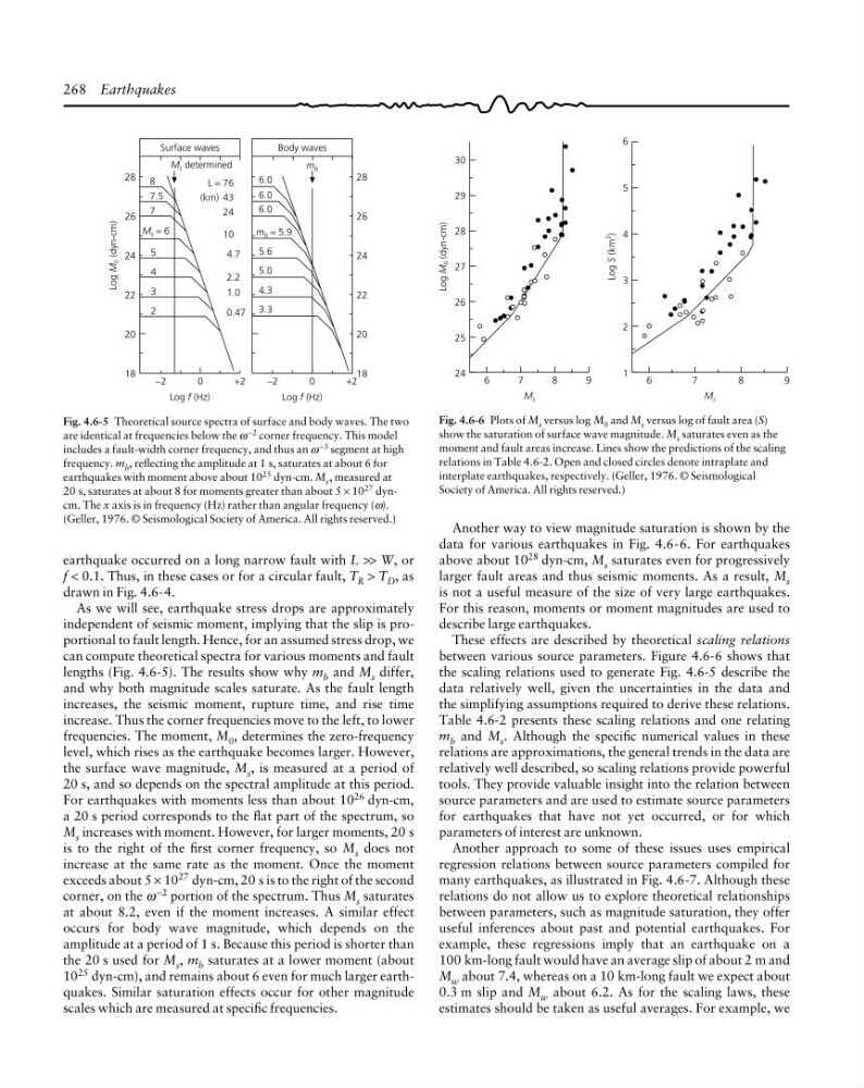
Fig. 4.6-5 Theoretical source spectra of surface and body waves. The two
are identical at frequencies below the ω
−2 corner frequency. This model
includes a fault-width corner frequency, and thus an ω
−3 segment at high
frequency. m b , reflecting the amplitude at 1 s, saturates at about 6 for
earthquakes with moment above about 10
25 dyn-cm. M s , measured at
20 s, saturates at about 8 for moments greater than about 5 × 10
27 dyncm. The x axis is in frequency (Hz) rather than angular frequency (ω).
(Geller, 1976. © Seismological Society of America. All rights reserved.)
6
Log M
0 (dyn-cm)
30
29
28
27
26
25
24
9
7
8
9
M s
6
Log S (km
2
)
6
5
4
3
2
1
7
8
M s
Fig. 4.6-6 Plots of M s versus log M 0 and M s versus log of fault area (S)
show the saturation of surface wave magnitude. M s saturates even as the
moment and fault areas increase. Lines show the predictions of the scaling
relations in Table 4.6-2. Open and closed circles denote intraplate and
interplate earthquakes, respectively. (Geller, 1976. © Seismological
Society of America. All rights reserved.)
earthquake occurred on a long narrow fault with L >> W, or
f < 0.1. Thus, in these cases or for a circular fault, T R > T D , as
drawn in Fig. 4.6-4.
As we will see, earthquake stress drops are approximately
independent of seismic moment, implying that the slip is proportional to fault length. Hence, for an assumed stress drop, we
can compute theoretical spectra for various moments and fault
lengths (Fig. 4.6-5). The results show why m b and M s differ,
and why both magnitude scales saturate. As the fault length
increases, the seismic moment, rupture time, and rise time
increase. Thus the corner frequencies move to the left, to lower
frequencies. The moment, M 0 , determines the zero-frequency
level, which rises as the earthquake becomes larger. However,
the surface wave magnitude, M s , is measured at a period of
20 s, and so depends on the spectral amplitude at this period.
For earthquakes with moments less than about 10 26 dyn-cm,
a 20 s period corresponds to the flat part of the spectrum, so
M s increases with moment. However, for larger moments, 20 s
is to the right of the first corner frequency, so M s does not
increase at the same rate as the moment. Once the moment
exceeds about 5 × 10
27 dyn-cm, 20 s is to the right of the second
corner, on the ω −2 portion of the spectrum. Thus M s saturates
at about 8.2, even if the moment increases. A similar effect
occurs for body wave magnitude, which depends on the
amplitude at a period of 1 s. Because this period is shorter than
the 20 s used for M s , m b saturates at a lower moment (about
10 25 dyn-cm), and remains about 6 even for much larger earthquakes. Similar saturation effects occur for other magnitude
scales which are measured at specific frequencies.
Another way to view magnitude saturation is shown by the
data for various earthquakes in Fig. 4.6-6. For earthquakes
above about 10 28 dyn-cm, M s saturates even for progressively
larger fault areas and thus seismic moments. As a result, M s
is not a useful measure of the size of very large earthquakes.
For this reason, moments or moment magnitudes are used to
describe large earthquakes.
These effects are described by theoretical scaling relations
between various source parameters. Figure 4.6-6 shows that
the scaling relations used to generate Fig. 4.6-5 describe the
data relatively well, given the uncertainties in the data and
the simplifying assumptions required to derive these relations.
Table 4.6-2 presents these scaling relations and one relating
m b and M s . Although the specific numerical values in these
relations are approximations, the general trends in the data are
relatively well described, so scaling relations provide powerful
tools. They provide valuable insight into the relation between
source parameters and are used to estimate source parameters
for earthquakes that have not yet occurred, or for which
parameters of interest are unknown.
Another approach to some of these issues uses empirical
regression relations between source parameters compiled for
many earthquakes, as illustrated in Fig. 4.6-7. Although these
relations do not allow us to explore theoretical relationships
between parameters, such as magnitude saturation, they offer
useful inferences about past and potential earthquakes. For
example, these regressions imply that an earthquake on a
100 km-long fault would have an average slip of about 2 m and
M w about 7.4, whereas on a 10 km-long fault we expect about
0.3 m slip and M w about 6.2. As for the scaling laws, these
estimates should be taken as useful averages. For example, we
Log M
0 (dyn-cm)
28
26
24
22
20
18
M s determined
8
7.5
7
M s = 6
5
4
3
2
L = 76
(km) 43
24
10
4.7
2.2
1.0
0.47
−2
0
+2
Log f (Hz)
−2
0
+2
Log f (Hz)
m b
28
26
24
22
20
18
Surface waves
Body waves
6.0
6.0
6.0
m b = 5.9
5.6
5.0
4.3
3.3
Fig. 4.6-5 Theoretical source spectra of surface and body waves. The two
are identical at frequencies below the ω
−2 corner frequency. This model
includes a fault-width corner frequency, and thus an ω
−3 segment at high
frequency. m b , reflecting the amplitude at 1 s, saturates at about 6 for
earthquakes with moment above about 10
25 dyn-cm. M s , measured at
20 s, saturates at about 8 for moments greater than about 5 × 10
27 dyncm. The x axis is in frequency (Hz) rather than angular frequency (ω).
(Geller, 1976. © Seismological Society of America. All rights reserved.)
6
Log M
0 (dyn-cm)
30
29
28
27
26
25
24
9
7
8
9
M s
6
Log S (km
2
)
6
5
4
3
2
1
7
8
M s
Fig. 4.6-6 Plots of M s versus log M 0 and M s versus log of fault area (S)
show the saturation of surface wave magnitude. M s saturates even as the
moment and fault areas increase. Lines show the predictions of the scaling
relations in Table 4.6-2. Open and closed circles denote intraplate and
interplate earthquakes, respectively. (Geller, 1976. © Seismological
Society of America. All rights reserved.)
earthquake occurred on a long narrow fault with L >> W, or
f < 0.1. Thus, in these cases or for a circular fault, T R > T D , as
drawn in Fig. 4.6-4.
As we will see, earthquake stress drops are approximately
independent of seismic moment, implying that the slip is proportional to fault length. Hence, for an assumed stress drop, we
can compute theoretical spectra for various moments and fault
lengths (Fig. 4.6-5). The results show why m b and M s differ,
and why both magnitude scales saturate. As the fault length
increases, the seismic moment, rupture time, and rise time
increase. Thus the corner frequencies move to the left, to lower
frequencies. The moment, M 0 , determines the zero-frequency
level, which rises as the earthquake becomes larger. However,
the surface wave magnitude, M s , is measured at a period of
20 s, and so depends on the spectral amplitude at this period.
For earthquakes with moments less than about 10 26 dyn-cm,
a 20 s period corresponds to the flat part of the spectrum, so
M s increases with moment. However, for larger moments, 20 s
is to the right of the first corner frequency, so M s does not
increase at the same rate as the moment. Once the moment
exceeds about 5 × 10
27 dyn-cm, 20 s is to the right of the second
corner, on the ω −2 portion of the spectrum. Thus M s saturates
at about 8.2, even if the moment increases. A similar effect
occurs for body wave magnitude, which depends on the
amplitude at a period of 1 s. Because this period is shorter than
the 20 s used for M s , m b saturates at a lower moment (about
10 25 dyn-cm), and remains about 6 even for much larger earthquakes. Similar saturation effects occur for other magnitude
scales which are measured at specific frequencies.
Another way to view magnitude saturation is shown by the
data for various earthquakes in Fig. 4.6-6. For earthquakes
above about 10 28 dyn-cm, M s saturates even for progressively
larger fault areas and thus seismic moments. As a result, M s
is not a useful measure of the size of very large earthquakes.
For this reason, moments or moment magnitudes are used to
describe large earthquakes.
These effects are described by theoretical scaling relations
between various source parameters. Figure 4.6-6 shows that
the scaling relations used to generate Fig. 4.6-5 describe the
data relatively well, given the uncertainties in the data and
the simplifying assumptions required to derive these relations.
Table 4.6-2 presents these scaling relations and one relating
m b and M s . Although the specific numerical values in these
relations are approximations, the general trends in the data are
relatively well described, so scaling relations provide powerful
tools. They provide valuable insight into the relation between
source parameters and are used to estimate source parameters
for earthquakes that have not yet occurred, or for which
parameters of interest are unknown.
Another approach to some of these issues uses empirical
regression relations between source parameters compiled for
many earthquakes, as illustrated in Fig. 4.6-7. Although these
relations do not allow us to explore theoretical relationships
between parameters, such as magnitude saturation, they offer
useful inferences about past and potential earthquakes. For
example, these regressions imply that an earthquake on a
100 km-long fault would have an average slip of about 2 m and
M w about 7.4, whereas on a 10 km-long fault we expect about
0.3 m slip and M w about 6.2. As for the scaling laws, these
estimates should be taken as useful averages. For example, we