

4.6 Source parameters 267
log | A(ω) | =
log
/
log
log ( / ) log
/
/
log
log (
/ )
log
/
M
T
M
T
T
T
M
TT
T
R
R
R
D
R D
D
0
0
0
2
2
2
2
4 2
2
ω
ω
ω
ω
ω
<
−
−
< <
−
−
<
⎧
⎨
⎪
⎩
⎪
⎫
⎬
⎪
⎭
⎪
(9)
This plot is divided into three regions by the frequencies 2/T R
and 2/T D , which are called corner frequencies. The spectrum
is flat for frequencies less than the first corner, goes as ω −1 between the corners, and decays as ω −2 for the high frequencies.
Thus the spectrum is parametrized by three factors: seismic
moment, rise time, and rupture time. It is worth noting that
other source spectral models have been used. A third corner
frequency can be added to this model, representing the effects
of fault width and yielding an ω −3 segment at high frequency.
Other models have a single corner frequency (dashed line in
Fig. 4.6-4, bottom) that combines the effects of rise and rupture
time. As a result, the interpretation of observed earthquake
spectra depends somewhat on the source model.
To see how the source spectrum varies with earthquake size,
we first note that the seismic moment is the scale factor for the
spectral amplitude at low frequencies ω → 0. This is the reason
why it is also called the “static” moment. It is defined (Section
4.2.3) as the product of the rigidity at the source depth, µ, the
average slip (or dislocation) on the fault, C, and the fault area,
S. The fault area can be written in terms of a shape factor f and
the square of a dimension L, so
M 0 = µCS = µCf L 2 .
(10)
For large earthquakes, faults are often treated as approximately rectangular, so L is the length, and f is the ratio of width
to length. Another common approach uses a circular fault
model for which L is the radius and f = π.
The rupture time (Eqn 4.3.8) needed for the rupture to
propagate along the fault is approximately
T R = L/v R = L/(0.7β),
(11)
if we assume that the rupture velocity is about 0.7 times the
shear velocity. The rise time needed for the dislocation to reach
its full value at any point on the fault has been predicted to be
about
T D = µC/(β∆σ) = 16Lf 1/2 /(7βπ 1.5 ),
(12)
where ∆σ is the stress drop in the earthquake, a quantity that
we will discuss shortly. Assuming a shear velocity of about
4 km/s, Eqns 11 and 12 yield approximately
T R = 0.35L, T D = 0.1Lf 1/2 .
(13)
Table 4.6-1 shows that the Truckee and San Fernando earthquakes occurred on approximately square faults (f = 1), Loma
Prieta and Alaska had L ≈ 2W, or f ≈ 0.5, and the San Francisco
Fig. 4.6-4 Top: The approximation to the (sin x)/x function used in
modeling the source spectrum. Bottom: Theoretical source spectrum of
an earthquake, modeled as three regions with slopes of 1, ω
−1
, and ω
−2 ,
divided by angular frequencies corresponding to the rupture and rise
times, T R and T D . Another common approximation uses a single corner
frequency, f c , at the intersection of the first and third spectrum segments.
The flat segment extending to zero frequency gives M 0 .
Log A( )
ω
1
0.8
0.6
0.4
0.2
0
0
0.5
1
1.5
2
2.5
3
sin x
x
1
1/x
x < 1
x > 1
fc
Slope = 1
Slope = 1/ω
Slope = 1/ω
2
2/T R
2/T D
Log ω
This function, sometimes written as sinc x = (sin x)/x, appears
in many applications in which only part of a signal is selected.
In Section 2.5.10 it described the amplitude resulting when part
of a plane wave diffracts through a slit. In Section 6.3, we will
use it to describe the effect on a time series spectrum from using
only part of the series. Here, the sinc function describes the fact
that the source pulse has finite duration.
Thus the spectral amplitude of the source signal is the product of the seismic moment and two sinc terms,
|
|
A
M
T
T
T
T
R
R
D
D
( )
sin(
/ )
/
sin(
/ )
/
,
ω
ω
ω
ω
ω
= 0
2
2
2
2
(7)
where T R and T D are the rupture and rise times. Often, we use
the logarithm of Eqn 7,
log A(ω) = log M 0 + log [sinc (ωT R /2)] + log [sinc (ωT D /2)].
(8)
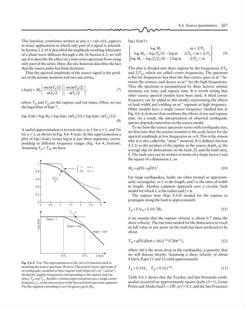
A useful approximation is to treat sinc x as 1 for x < 1, and 1/x
for x > 1, as shown in Fig. 4.6-4 (top). In this approximation a
plot of log | A(ω) | versus log ω is just three segments, corresponding to different frequency ranges (Fig. 4.6-4, bottom).
Assuming T R > T D , we have
log | A(ω) | =
log
/
log
log ( / ) log
/
/
log
log (
/ )
log
/
M
T
M
T
T
T
M
TT
T
R
R
R
D
R D
D
0
0
0
2
2
2
2
4 2
2
ω
ω
ω
ω
ω
<
−
−
< <
−
−
<
⎧
⎨
⎪
⎩
⎪
⎫
⎬
⎪
⎭
⎪
(9)
This plot is divided into three regions by the frequencies 2/T R
and 2/T D , which are called corner frequencies. The spectrum
is flat for frequencies less than the first corner, goes as ω −1 between the corners, and decays as ω −2 for the high frequencies.
Thus the spectrum is parametrized by three factors: seismic
moment, rise time, and rupture time. It is worth noting that
other source spectral models have been used. A third corner
frequency can be added to this model, representing the effects
of fault width and yielding an ω −3 segment at high frequency.
Other models have a single corner frequency (dashed line in
Fig. 4.6-4, bottom) that combines the effects of rise and rupture
time. As a result, the interpretation of observed earthquake
spectra depends somewhat on the source model.
To see how the source spectrum varies with earthquake size,
we first note that the seismic moment is the scale factor for the
spectral amplitude at low frequencies ω → 0. This is the reason
why it is also called the “static” moment. It is defined (Section
4.2.3) as the product of the rigidity at the source depth, µ, the
average slip (or dislocation) on the fault, C, and the fault area,
S. The fault area can be written in terms of a shape factor f and
the square of a dimension L, so
M 0 = µCS = µCf L 2 .
(10)
For large earthquakes, faults are often treated as approximately rectangular, so L is the length, and f is the ratio of width
to length. Another common approach uses a circular fault
model for which L is the radius and f = π.
The rupture time (Eqn 4.3.8) needed for the rupture to
propagate along the fault is approximately
T R = L/v R = L/(0.7β),
(11)
if we assume that the rupture velocity is about 0.7 times the
shear velocity. The rise time needed for the dislocation to reach
its full value at any point on the fault has been predicted to be
about
T D = µC/(β∆σ) = 16Lf 1/2 /(7βπ 1.5 ),
(12)
where ∆σ is the stress drop in the earthquake, a quantity that
we will discuss shortly. Assuming a shear velocity of about
4 km/s, Eqns 11 and 12 yield approximately
T R = 0.35L, T D = 0.1Lf 1/2 .
(13)
Table 4.6-1 shows that the Truckee and San Fernando earthquakes occurred on approximately square faults (f = 1), Loma
Prieta and Alaska had L ≈ 2W, or f ≈ 0.5, and the San Francisco
Fig. 4.6-4 Top: The approximation to the (sin x)/x function used in
modeling the source spectrum. Bottom: Theoretical source spectrum of
an earthquake, modeled as three regions with slopes of 1, ω
−1
, and ω
−2 ,
divided by angular frequencies corresponding to the rupture and rise
times, T R and T D . Another common approximation uses a single corner
frequency, f c , at the intersection of the first and third spectrum segments.
The flat segment extending to zero frequency gives M 0 .
Log A( )
ω
1
0.8
0.6
0.4
0.2
0
0
0.5
1
1.5
2
2.5
3
sin x
x
1
1/x
x < 1
x > 1
fc
Slope = 1
Slope = 1/ω
Slope = 1/ω
2
2/T R
2/T D
Log ω
This function, sometimes written as sinc x = (sin x)/x, appears
in many applications in which only part of a signal is selected.
In Section 2.5.10 it described the amplitude resulting when part
of a plane wave diffracts through a slit. In Section 6.3, we will
use it to describe the effect on a time series spectrum from using
only part of the series. Here, the sinc function describes the fact
that the source pulse has finite duration.
Thus the spectral amplitude of the source signal is the product of the seismic moment and two sinc terms,
|
|
A
M
T
T
T
T
R
R
D
D
( )
sin(
/ )
/
sin(
/ )
/
,
ω
ω
ω
ω
ω
= 0
2
2
2
2
(7)
where T R and T D are the rupture and rise times. Often, we use
the logarithm of Eqn 7,
log A(ω) = log M 0 + log [sinc (ωT R /2)] + log [sinc (ωT D /2)].
(8)
A useful approximation is to treat sinc x as 1 for x < 1, and 1/x
for x > 1, as shown in Fig. 4.6-4 (top). In this approximation a
plot of log | A(ω) | versus log ω is just three segments, corresponding to different frequency ranges (Fig. 4.6-4, bottom).
Assuming T R > T D , we have