

266 Earthquakes
San
Fernando,
1971
San
Francisco,
1906
M 0 = 1.2 × 10
26
M 0 = 5.4 × 10
27
M s = 6.6
M s = 7.8
Slip = 1.4 m
Slip = 4 m
Alaska,1964
M 0 = 5.2 × 10
29
M s = 8.4
Slip = 7 m
100 km
M 0 =
2.4 × 10
30
M s = 8.3
Slip = 21 m
Chile, 1960
are assumed, and which are inferred by combining others. For
example, the relation between the seismic moment, slip, and
fault dimensions depends on the rigidity assumed (typically 3–
5 × 10 11 dyn/cm 2 for shallow earthquakes). Even so, such data
are sufficient to show the basic effects of interest.
We can understand these effects given what we have discussed about the amplitudes of body and surface waves in
Sections 4.2 and 4.3 — information that was not available to
seismologists when these magnitude scales were developed. We
have seen that the amplitudes depend on the scalar moment,
the azimuth of a seismometer relative to the fault geometry, the
distance from the source, and the source depth. Moreover,
because the source time function has a finite duration, depending on fault dimensions and rise time, the amplitudes vary
with frequency. We will see shortly that these frequency variations explain the differences between magnitudes and their
saturation.
Before doing so, we note the simple and elegant solution that
has been adopted: namely, defining a magnitude scale based on
the seismic moment. The moment magnitude,
M
M
w =
−
log
.
. ,
0
1 5
10 73
(5)
defined for M 0 in dyn-cm, has several advantages. It gives a
magnitude directly tied to earthquake source processes that
does not saturate. Moreover, it preserves the simplicity of the
magnitude scale by giving values of order 1 compatible with
other magnitude scales. As we will see, M w is comparable to M s
until M s saturates at about 8.2, but then increases. The largest
seismically recorded earthquake, the 1960 Chile event listed
in Table 4.6-1, had M w 9.5. Moment magnitude has become
the common measure of the magnitude of large earthquakes.
Estimation of M 0 (and therefore M w ) requires more analysis of
seismograms than for m b or M s . However, semi-automated
programs like the Harvard CMT project or comparable regional analyses now regularly compute moment magnitudes
for most earthquakes larger than about M w 5.
4.6.2 Source spectra and scaling laws
The relations between the moment and various magnitudes
arise from the spectrum of the radiated seismic waves. We saw
in Section 4.3.2 that the radiated waves depend on the product
of the scalar moment and the source time function generated by
the earthquake. We used a simple model in which the time
function was the convolution of two “boxcar” time functions
due to the finite length of the fault and the finite rise time of the
faulting at any point. The Fourier transform of the resulting
time function is the product of the transforms of the boxcars.
The transform of a boxcar of height 1/T and length T is
F
T
e dt
Ti
e
e
T
T
T
T
i t
i T
i T
( )
(
)
sin( / )
/
.
/
/
/
/
ω
ω
ω
ω
ω
ω
ω
=
=
−
=
−
−
Ύ
2
2
2
2
1
1
2
2
(6)
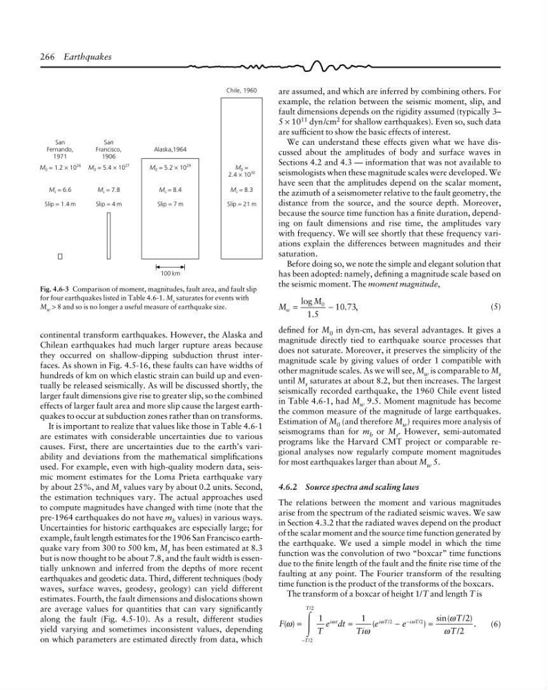
Fig. 4.6-3 Comparison of moment, magnitudes, fault area, and fault slip
for four earthquakes listed in Table 4.6-1. M s saturates for events with
M w > 8 and so is no longer a useful measure of earthquake size.
continental transform earthquakes. However, the Alaska and
Chilean earthquakes had much larger rupture areas because
they occurred on shallow-dipping subduction thrust interfaces. As shown in Fig. 4.5-16, these faults can have widths of
hundreds of km on which elastic strain can build up and eventually be released seismically. As will be discussed shortly, the
larger fault dimensions give rise to greater slip, so the combined
effects of larger fault area and more slip cause the largest earthquakes to occur at subduction zones rather than on transforms.
It is important to realize that values like those in Table 4.6-1
are estimates with considerable uncertainties due to various
causes. First, there are uncertainties due to the earth’s variability and deviations from the mathematical simplifications
used. For example, even with high-quality modern data, seismic moment estimates for the Loma Prieta earthquake vary
by about 25%, and M s values vary by about 0.2 units. Second,
the estimation techniques vary. The actual approaches used
to compute magnitudes have changed with time (note that the
pre-1964 earthquakes do not have m b values) in various ways.
Uncertainties for historic earthquakes are especially large; for
example, fault length estimates for the 1906 San Francisco earthquake vary from 300 to 500 km, M s has been estimated at 8.3
but is now thought to be about 7.8, and the fault width is essentially unknown and inferred from the depths of more recent
earthquakes and geodetic data. Third, different techniques (body
waves, surface waves, geodesy, geology) can yield different
estimates. Fourth, the fault dimensions and dislocations shown
are average values for quantities that can vary significantly
along the fault (Fig. 4.5-10). As a result, different studies
yield varying and sometimes inconsistent values, depending
on which parameters are estimated directly from data, which
San
Fernando,
1971
San
Francisco,
1906
M 0 = 1.2 × 10
26
M 0 = 5.4 × 10
27
M s = 6.6
M s = 7.8
Slip = 1.4 m
Slip = 4 m
Alaska,1964
M 0 = 5.2 × 10
29
M s = 8.4
Slip = 7 m
100 km
M 0 =
2.4 × 10
30
M s = 8.3
Slip = 21 m
Chile, 1960
are assumed, and which are inferred by combining others. For
example, the relation between the seismic moment, slip, and
fault dimensions depends on the rigidity assumed (typically 3–
5 × 10 11 dyn/cm 2 for shallow earthquakes). Even so, such data
are sufficient to show the basic effects of interest.
We can understand these effects given what we have discussed about the amplitudes of body and surface waves in
Sections 4.2 and 4.3 — information that was not available to
seismologists when these magnitude scales were developed. We
have seen that the amplitudes depend on the scalar moment,
the azimuth of a seismometer relative to the fault geometry, the
distance from the source, and the source depth. Moreover,
because the source time function has a finite duration, depending on fault dimensions and rise time, the amplitudes vary
with frequency. We will see shortly that these frequency variations explain the differences between magnitudes and their
saturation.
Before doing so, we note the simple and elegant solution that
has been adopted: namely, defining a magnitude scale based on
the seismic moment. The moment magnitude,
M
M
w =
−
log
.
. ,
0
1 5
10 73
(5)
defined for M 0 in dyn-cm, has several advantages. It gives a
magnitude directly tied to earthquake source processes that
does not saturate. Moreover, it preserves the simplicity of the
magnitude scale by giving values of order 1 compatible with
other magnitude scales. As we will see, M w is comparable to M s
until M s saturates at about 8.2, but then increases. The largest
seismically recorded earthquake, the 1960 Chile event listed
in Table 4.6-1, had M w 9.5. Moment magnitude has become
the common measure of the magnitude of large earthquakes.
Estimation of M 0 (and therefore M w ) requires more analysis of
seismograms than for m b or M s . However, semi-automated
programs like the Harvard CMT project or comparable regional analyses now regularly compute moment magnitudes
for most earthquakes larger than about M w 5.
4.6.2 Source spectra and scaling laws
The relations between the moment and various magnitudes
arise from the spectrum of the radiated seismic waves. We saw
in Section 4.3.2 that the radiated waves depend on the product
of the scalar moment and the source time function generated by
the earthquake. We used a simple model in which the time
function was the convolution of two “boxcar” time functions
due to the finite length of the fault and the finite rise time of the
faulting at any point. The Fourier transform of the resulting
time function is the product of the transforms of the boxcars.
The transform of a boxcar of height 1/T and length T is
F
T
e dt
Ti
e
e
T
T
T
T
i t
i T
i T
( )
(
)
sin( / )
/
.
/
/
/
/
ω
ω
ω
ω
ω
ω
ω
=
=
−
=
−
−
Ύ
2
2
2
2
1
1
2
2
(6)
Fig. 4.6-3 Comparison of moment, magnitudes, fault area, and fault slip
for four earthquakes listed in Table 4.6-1. M s saturates for events with
M w > 8 and so is no longer a useful measure of earthquake size.
continental transform earthquakes. However, the Alaska and
Chilean earthquakes had much larger rupture areas because
they occurred on shallow-dipping subduction thrust interfaces. As shown in Fig. 4.5-16, these faults can have widths of
hundreds of km on which elastic strain can build up and eventually be released seismically. As will be discussed shortly, the
larger fault dimensions give rise to greater slip, so the combined
effects of larger fault area and more slip cause the largest earthquakes to occur at subduction zones rather than on transforms.
It is important to realize that values like those in Table 4.6-1
are estimates with considerable uncertainties due to various
causes. First, there are uncertainties due to the earth’s variability and deviations from the mathematical simplifications
used. For example, even with high-quality modern data, seismic moment estimates for the Loma Prieta earthquake vary
by about 25%, and M s values vary by about 0.2 units. Second,
the estimation techniques vary. The actual approaches used
to compute magnitudes have changed with time (note that the
pre-1964 earthquakes do not have m b values) in various ways.
Uncertainties for historic earthquakes are especially large; for
example, fault length estimates for the 1906 San Francisco earthquake vary from 300 to 500 km, M s has been estimated at 8.3
but is now thought to be about 7.8, and the fault width is essentially unknown and inferred from the depths of more recent
earthquakes and geodetic data. Third, different techniques (body
waves, surface waves, geodesy, geology) can yield different
estimates. Fourth, the fault dimensions and dislocations shown
are average values for quantities that can vary significantly
along the fault (Fig. 4.5-10). As a result, different studies
yield varying and sometimes inconsistent values, depending
on which parameters are estimated directly from data, which