

4.6 Source parameters 265
40
D
is
ta
n
c
e
(°
)
Q(h, ∆)
6
5
4
3
30
20
10
100
200
300
400
500
600
700
De pt h of ea rth qu ak e (km )
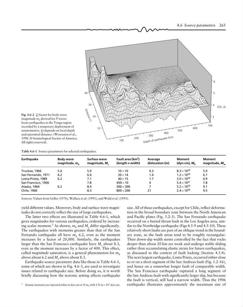
Fig. 4.6-2 Q factor for body wave
magnitude m b derived for P waves
from earthquakes in the Tonga region
recorded by a temporary deployment of
seismometers. Q depends on focal depth
and epicentral distance. (Wysession et al.,
1996. © Seismological Society of America.
All rights reserved).
3 Seismic moments are reported either in dyn-cm or N-m, with 1 N-m = 10 7 dyn-cm.
size. All of these earthquakes, except for Chile, reflect deformation in the broad boundary zone between the North American
and Pacific plates (Fig. 5.2-3). The San Fernando earthquake
occurred on a buried thrust fault in the Los Angeles area, similar to the Northridge earthquake (Figs 4.5-9 and 4.5-10). These
relatively short faults are part of an oblique trend in the boundary zone, so the fault areas tend to be roughly rectangular.
Their down-dip width seems controlled by the fact that rocks
deeper than about 20 km are weak and undergo stable sliding
rather than accumulating elastic strain for future earthquakes,
as discussed in the context of fault locking (Section 4.5.4).
The next largest earthquake, Loma Prieta, occurred either close
to or on a short segment of the San Andreas fault (Fig. 1.2-16),
and hence on a somewhat longer fault of comparable width.
The San Francisco earthquake ruptured a long segment of
the San Andreas fault with significantly larger slip, but because
the fault is vertical, still had a narrow width. Thus the 1906
earthquake illustrates approximately the maximum size of
yield different values. Moreover, body and surface wave magnitudes do not correctly reflect the size of large earthquakes.
The latter two effects are illustrated in Table 4.6-1, which
gives magnitudes for various earthquakes, ordered by increasing scalar moment. 3 As shown, m b and M s differ significantly.
The earthquakes with moments greater than that of the San
Fernando earthquake all have m b 6.2, even as the moment
increases by a factor of 20,000. Similarly, the earthquakes
larger than the San Francisco earthquake have M s about 8.3,
even as the moment increases by a factor of 400. This effect,
called magnitude saturation, is a general phenomenon for m b
above about 6.2 and M s above about 8.3.
Earthquake source parameter data like those in Table 4.6-1,
some of which are shown in Fig. 4.6-3, are used to investigate
issues related to earthquake size. Before doing so, it is worth
briefly discussing how the tectonic setting affects earthquake
Table 4.6-1 Source parameters for selected earthquakes.
Earthquake
Body wave
Surface wave
Fault area (km
2 )
Average
Moment
Moment
magnitude, m b
magnitude, M s
(length ×
× ×
× × width)
dislocation (m)
(dyn-cm), M 0
magnitude, M w
Truckee, 1966
5.4
5.9
10 × 10
0.3
8.3 × 10
24
5.9
San Fernando, 1971
6.2
6.6
20 × 14
1.4
1.2 × 10
26
6.7
Loma Prieta, 1989
6.2
7.1
40 × 15
1.7
3.0 × 10
26
6.9
San Francisco, 1906
7.8
450 × 10
4
5.4 × 10
27
7.8
Alaska, 1964
6.2
8.4
500 × 300
7
5.2 × 10 29
9.1
Chile, 1960
8.3
800 × 200
21
2.4 × 10
30
9.5
Sources: Values from Geller (1976), Wallace et al. (1991), and Wald et al. (1993).
40
D
is
ta
n
c
e
(°
)
Q(h, ∆)
6
5
4
3
30
20
10
100
200
300
400
500
600
700
De pt h of ea rth qu ak e (km )
Fig. 4.6-2 Q factor for body wave
magnitude m b derived for P waves
from earthquakes in the Tonga region
recorded by a temporary deployment of
seismometers. Q depends on focal depth
and epicentral distance. (Wysession et al.,
1996. © Seismological Society of America.
All rights reserved).
3 Seismic moments are reported either in dyn-cm or N-m, with 1 N-m = 10 7 dyn-cm.
size. All of these earthquakes, except for Chile, reflect deformation in the broad boundary zone between the North American
and Pacific plates (Fig. 5.2-3). The San Fernando earthquake
occurred on a buried thrust fault in the Los Angeles area, similar to the Northridge earthquake (Figs 4.5-9 and 4.5-10). These
relatively short faults are part of an oblique trend in the boundary zone, so the fault areas tend to be roughly rectangular.
Their down-dip width seems controlled by the fact that rocks
deeper than about 20 km are weak and undergo stable sliding
rather than accumulating elastic strain for future earthquakes,
as discussed in the context of fault locking (Section 4.5.4).
The next largest earthquake, Loma Prieta, occurred either close
to or on a short segment of the San Andreas fault (Fig. 1.2-16),
and hence on a somewhat longer fault of comparable width.
The San Francisco earthquake ruptured a long segment of
the San Andreas fault with significantly larger slip, but because
the fault is vertical, still had a narrow width. Thus the 1906
earthquake illustrates approximately the maximum size of
yield different values. Moreover, body and surface wave magnitudes do not correctly reflect the size of large earthquakes.
The latter two effects are illustrated in Table 4.6-1, which
gives magnitudes for various earthquakes, ordered by increasing scalar moment. 3 As shown, m b and M s differ significantly.
The earthquakes with moments greater than that of the San
Fernando earthquake all have m b 6.2, even as the moment
increases by a factor of 20,000. Similarly, the earthquakes
larger than the San Francisco earthquake have M s about 8.3,
even as the moment increases by a factor of 400. This effect,
called magnitude saturation, is a general phenomenon for m b
above about 6.2 and M s above about 8.3.
Earthquake source parameter data like those in Table 4.6-1,
some of which are shown in Fig. 4.6-3, are used to investigate
issues related to earthquake size. Before doing so, it is worth
briefly discussing how the tectonic setting affects earthquake
Table 4.6-1 Source parameters for selected earthquakes.
Earthquake
Body wave
Surface wave
Fault area (km
2 )
Average
Moment
Moment
magnitude, m b
magnitude, M s
(length ×
× ×
× × width)
dislocation (m)
(dyn-cm), M 0
magnitude, M w
Truckee, 1966
5.4
5.9
10 × 10
0.3
8.3 × 10
24
5.9
San Fernando, 1971
6.2
6.6
20 × 14
1.4
1.2 × 10
26
6.7
Loma Prieta, 1989
6.2
7.1
40 × 15
1.7
3.0 × 10
26
6.9
San Francisco, 1906
7.8
450 × 10
4
5.4 × 10
27
7.8
Alaska, 1964
6.2
8.4
500 × 300
7
5.2 × 10 29
9.1
Chile, 1960
8.3
800 × 200
21
2.4 × 10
30
9.5
Sources: Values from Geller (1976), Wallace et al. (1991), and Wald et al. (1993).