

260 Earthquakes
the right side near the fault is retarded during the interseismic
period, and then “catches up” to the far-field motion due to the
coseismic deformation. Equations 4 and 6 are thus mathematical formulations of the elastic rebound model in Fig. 4.1-3.
If the fault is a plate boundary, the interseismic deformation
occurs over a finite plate boundary zone within which sites on
either side of the boundary move relative to the interior of the
plate they are on. In this case, the boundary zone is relatively
narrow, comparable to the depth to which the fault is locked.
However, as we will see, many plate boundary zones are
broader because additional faults take up some of the plate
motion.
Because the interseismic motion is the difference between the
far-field motion and coseismic deformation, its variation with
distance from the fault depends on the locking depth and farfield rate. Comparison with the coseismic slip shows that the
width of the zone across which the motion changes rapidly
depends on the locking depth. Shallow locking concentrates
interseismic slip near the fault, whereas deeper locking spreads
it out into a broad shear zone. Hence a series of geodetic
surveys can develop a velocity profile across the fault, which
we can interpret by setting D = vt in Eqn 6 and dividing the
change in positions between surveys by the time between them.
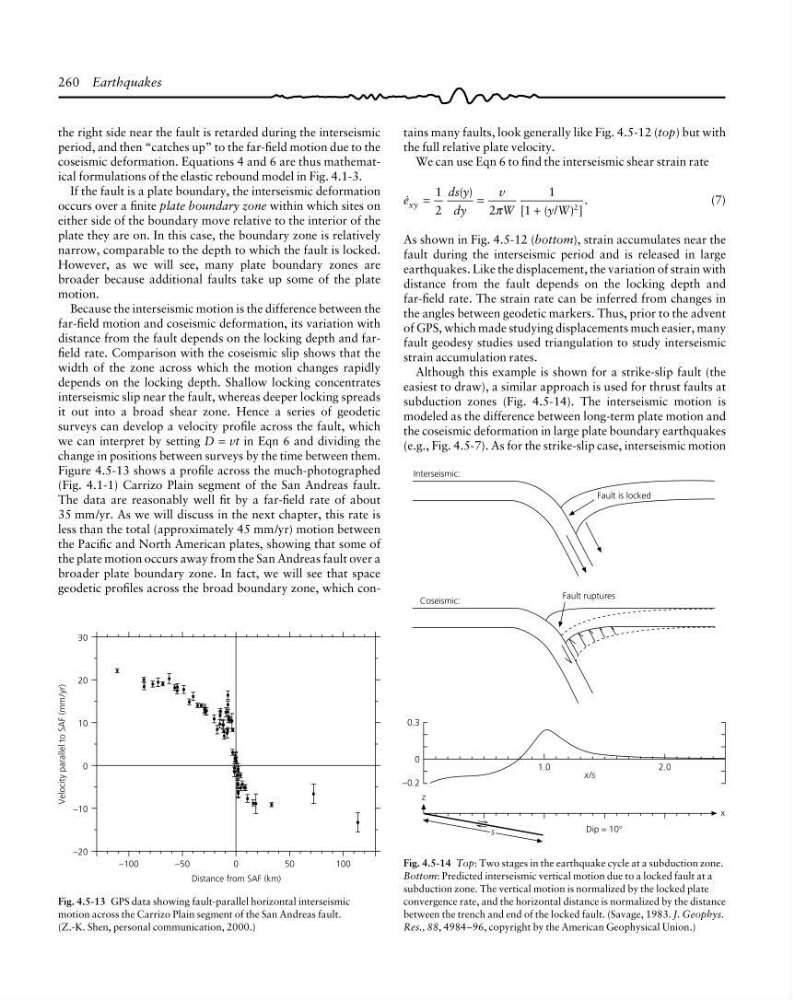
Figure 4.5-13 shows a profile across the much-photographed
(Fig. 4.1-1) Carrizo Plain segment of the San Andreas fault.
The data are reasonably well fit by a far-field rate of about
35 mm/yr. As we will discuss in the next chapter, this rate is
less than the total (approximately 45 mm/yr) motion between
the Pacific and North American plates, showing that some of
the plate motion occurs away from the San Andreas fault over a
broader plate boundary zone. In fact, we will see that space
geodetic profiles across the broad boundary zone, which conFig. 4.5-13 GPS data showing fault-parallel horizontal interseismic
motion across the Carrizo Plain segment of the San Andreas fault.
(Z.-K. Shen, personal communication, 2000.)
30
20
10
0
−10
−20
Velocity parallel to SAF (mm/yr)
−100
−50
0
50
100
Distance from SAF (km)
Fig. 4.5-14 Top: Two stages in the earthquake cycle at a subduction zone.
Bottom: Predicted interseismic vertical motion due to a locked fault at a
subduction zone. The vertical motion is normalized by the locked plate
convergence rate, and the horizontal distance is normalized by the distance
between the trench and end of the locked fault. (Savage, 1983. J. Geophys.
Res., 88, 4984–96, copyright by the American Geophysical Union.)
0.3
0
−0.2
1.0
2.0
x/s
z
Dip = 10°
s
x
Coseismic:
Fault ruptures
Interseismic:
Fault is locked
tains many faults, look generally like Fig. 4.5-12 (top) but with
the full relative plate velocity.
We can use Eqn 6 to find the interseismic shear strain rate
G xy =
=
+
( )
[
( / ) ]
.
1
2
2
1
1
2
ds y
dy
v
W
yW
π
(7)
As shown in Fig. 4.5-12 (bottom), strain accumulates near the
fault during the interseismic period and is released in large
earthquakes. Like the displacement, the variation of strain with
distance from the fault depends on the locking depth and
far-field rate. The strain rate can be inferred from changes in
the angles between geodetic markers. Thus, prior to the advent
of GPS, which made studying displacements much easier, many
fault geodesy studies used triangulation to study interseismic
strain accumulation rates.
Although this example is shown for a strike-slip fault (the
easiest to draw), a similar approach is used for thrust faults at
subduction zones (Fig. 4.5-14). The interseismic motion is
modeled as the difference between long-term plate motion and
the coseismic deformation in large plate boundary earthquakes
(e.g., Fig. 4.5-7). As for the strike-slip case, interseismic motion
the right side near the fault is retarded during the interseismic
period, and then “catches up” to the far-field motion due to the
coseismic deformation. Equations 4 and 6 are thus mathematical formulations of the elastic rebound model in Fig. 4.1-3.
If the fault is a plate boundary, the interseismic deformation
occurs over a finite plate boundary zone within which sites on
either side of the boundary move relative to the interior of the
plate they are on. In this case, the boundary zone is relatively
narrow, comparable to the depth to which the fault is locked.
However, as we will see, many plate boundary zones are
broader because additional faults take up some of the plate
motion.
Because the interseismic motion is the difference between the
far-field motion and coseismic deformation, its variation with
distance from the fault depends on the locking depth and farfield rate. Comparison with the coseismic slip shows that the
width of the zone across which the motion changes rapidly
depends on the locking depth. Shallow locking concentrates
interseismic slip near the fault, whereas deeper locking spreads
it out into a broad shear zone. Hence a series of geodetic
surveys can develop a velocity profile across the fault, which
we can interpret by setting D = vt in Eqn 6 and dividing the
change in positions between surveys by the time between them.
Figure 4.5-13 shows a profile across the much-photographed
(Fig. 4.1-1) Carrizo Plain segment of the San Andreas fault.
The data are reasonably well fit by a far-field rate of about
35 mm/yr. As we will discuss in the next chapter, this rate is
less than the total (approximately 45 mm/yr) motion between
the Pacific and North American plates, showing that some of
the plate motion occurs away from the San Andreas fault over a
broader plate boundary zone. In fact, we will see that space
geodetic profiles across the broad boundary zone, which conFig. 4.5-13 GPS data showing fault-parallel horizontal interseismic
motion across the Carrizo Plain segment of the San Andreas fault.
(Z.-K. Shen, personal communication, 2000.)
30
20
10
0
−10
−20
Velocity parallel to SAF (mm/yr)
−100
−50
0
50
100
Distance from SAF (km)
Fig. 4.5-14 Top: Two stages in the earthquake cycle at a subduction zone.
Bottom: Predicted interseismic vertical motion due to a locked fault at a
subduction zone. The vertical motion is normalized by the locked plate
convergence rate, and the horizontal distance is normalized by the distance
between the trench and end of the locked fault. (Savage, 1983. J. Geophys.
Res., 88, 4984–96, copyright by the American Geophysical Union.)
0.3
0
−0.2
1.0
2.0
x/s
z
Dip = 10°
s
x
Coseismic:
Fault ruptures
Interseismic:
Fault is locked
tains many faults, look generally like Fig. 4.5-12 (top) but with
the full relative plate velocity.
We can use Eqn 6 to find the interseismic shear strain rate
G xy =
=
+
( )
[
( / ) ]
.
1
2
2
1
1
2
ds y
dy
v
W
yW
π
(7)
As shown in Fig. 4.5-12 (bottom), strain accumulates near the
fault during the interseismic period and is released in large
earthquakes. Like the displacement, the variation of strain with
distance from the fault depends on the locking depth and
far-field rate. The strain rate can be inferred from changes in
the angles between geodetic markers. Thus, prior to the advent
of GPS, which made studying displacements much easier, many
fault geodesy studies used triangulation to study interseismic
strain accumulation rates.
Although this example is shown for a strike-slip fault (the
easiest to draw), a similar approach is used for thrust faults at
subduction zones (Fig. 4.5-14). The interseismic motion is
modeled as the difference between long-term plate motion and
the coseismic deformation in large plate boundary earthquakes
(e.g., Fig. 4.5-7). As for the strike-slip case, interseismic motion