

258 Earthquakes
Depth (km)
5
7.5
10
12.5
15
17.5
20
a. Strong motion
0
5
10
15
Slip (m)
5
7.5
10
12.5
15
17.5
20
b. Teleseismic
0
5
10
15
0.8
0.4
2
1
Depth (km)
5
7.5
10
12.5
15
17.5
20
c. Geodetic
1
.
6
0
5
10
15
5
7.5
10
12.5
15
17.5
20
d. Combined
1 .2
0
5
10
15
0.8
0.4
0.4
1.6
1.2
0.8
1 .2
1.6
*
*
0 .8
2
1
.
2
0 .4
*
2.4
1 .6
2
2
.4
Distance along strike (km)
Distance along strike (km)
*
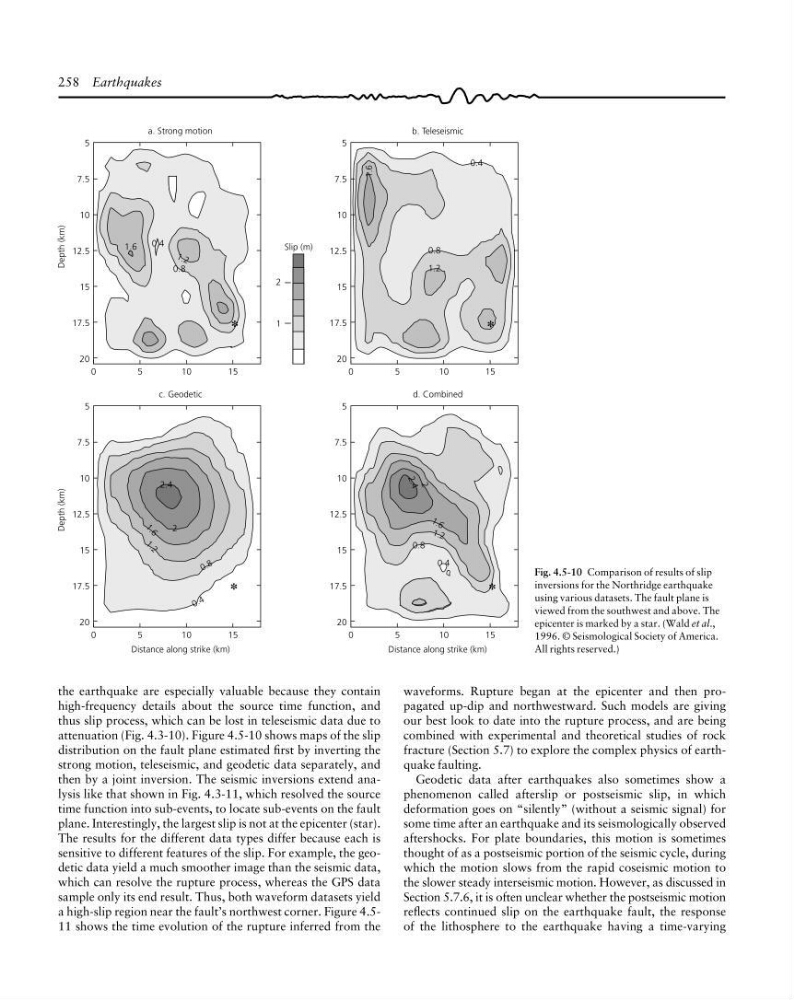
Fig. 4.5-10 Comparison of results of slip
inversions for the Northridge earthquake
using various datasets. The fault plane is
viewed from the southwest and above. The
epicenter is marked by a star. (Wald et al.,
1996. © Seismological Society of America.
All rights reserved.)
waveforms. Rupture began at the epicenter and then propagated up-dip and northwestward. Such models are giving
our best look to date into the rupture process, and are being
combined with experimental and theoretical studies of rock
fracture (Section 5.7) to explore the complex physics of earthquake faulting.
Geodetic data after earthquakes also sometimes show a
phenomenon called afterslip or postseismic slip, in which
deformation goes on “silently” (without a seismic signal) for
some time after an earthquake and its seismologically observed
aftershocks. For plate boundaries, this motion is sometimes
thought of as a postseismic portion of the seismic cycle, during
which the motion slows from the rapid coseismic motion to
the slower steady interseismic motion. However, as discussed in
Section 5.7.6, it is often unclear whether the postseismic motion
reflects continued slip on the earthquake fault, the response
of the lithosphere to the earthquake having a time-varying
the earthquake are especially valuable because they contain
high-frequency details about the source time function, and
thus slip process, which can be lost in teleseismic data due to
attenuation (Fig. 4.3-10). Figure 4.5-10 shows maps of the slip
distribution on the fault plane estimated first by inverting the
strong motion, teleseismic, and geodetic data separately, and
then by a joint inversion. The seismic inversions extend analysis like that shown in Fig. 4.3-11, which resolved the source
time function into sub-events, to locate sub-events on the fault
plane. Interestingly, the largest slip is not at the epicenter (star).
The results for the different data types differ because each is
sensitive to different features of the slip. For example, the geodetic data yield a much smoother image than the seismic data,
which can resolve the rupture process, whereas the GPS data
sample only its end result. Thus, both waveform datasets yield
a high-slip region near the fault’s northwest corner. Figure 4.511 shows the time evolution of the rupture inferred from the
Depth (km)
5
7.5
10
12.5
15
17.5
20
a. Strong motion
0
5
10
15
Slip (m)
5
7.5
10
12.5
15
17.5
20
b. Teleseismic
0
5
10
15
0.8
0.4
2
1
Depth (km)
5
7.5
10
12.5
15
17.5
20
c. Geodetic
1
.
6
0
5
10
15
5
7.5
10
12.5
15
17.5
20
d. Combined
1 .2
0
5
10
15
0.8
0.4
0.4
1.6
1.2
0.8
1 .2
1.6
*
*
0 .8
2
1
.
2
0 .4
*
2.4
1 .6
2
2
.4
Distance along strike (km)
Distance along strike (km)
*
Fig. 4.5-10 Comparison of results of slip
inversions for the Northridge earthquake
using various datasets. The fault plane is
viewed from the southwest and above. The
epicenter is marked by a star. (Wald et al.,
1996. © Seismological Society of America.
All rights reserved.)
waveforms. Rupture began at the epicenter and then propagated up-dip and northwestward. Such models are giving
our best look to date into the rupture process, and are being
combined with experimental and theoretical studies of rock
fracture (Section 5.7) to explore the complex physics of earthquake faulting.
Geodetic data after earthquakes also sometimes show a
phenomenon called afterslip or postseismic slip, in which
deformation goes on “silently” (without a seismic signal) for
some time after an earthquake and its seismologically observed
aftershocks. For plate boundaries, this motion is sometimes
thought of as a postseismic portion of the seismic cycle, during
which the motion slows from the rapid coseismic motion to
the slower steady interseismic motion. However, as discussed in
Section 5.7.6, it is often unclear whether the postseismic motion
reflects continued slip on the earthquake fault, the response
of the lithosphere to the earthquake having a time-varying
the earthquake are especially valuable because they contain
high-frequency details about the source time function, and
thus slip process, which can be lost in teleseismic data due to
attenuation (Fig. 4.3-10). Figure 4.5-10 shows maps of the slip
distribution on the fault plane estimated first by inverting the
strong motion, teleseismic, and geodetic data separately, and
then by a joint inversion. The seismic inversions extend analysis like that shown in Fig. 4.3-11, which resolved the source
time function into sub-events, to locate sub-events on the fault
plane. Interestingly, the largest slip is not at the epicenter (star).
The results for the different data types differ because each is
sensitive to different features of the slip. For example, the geodetic data yield a much smoother image than the seismic data,
which can resolve the rupture process, whereas the GPS data
sample only its end result. Thus, both waveform datasets yield
a high-slip region near the fault’s northwest corner. Figure 4.511 shows the time evolution of the rupture inferred from the