

0
5
−10
−15
−20
25
−10
−5
5
0
1 0
1 5
2 0
Mainshock
Distance (km)
Depth (km)
34.6
34.4
34.2
34
0
k m
2 0
10 cm
−118.8
−118.6
−118.4
−118.2
Longitude
Latitude
4.5 Earthquake geodesy 257
Displacement
0.5
0.4
0.3
0.2
0.1
V
I
II IV
VI
III
0
5
10
15
20
25
Distance (km)
Models I, V
10
Depth (km)
Models II, VI
10
Model III
10
Model IV
10
20
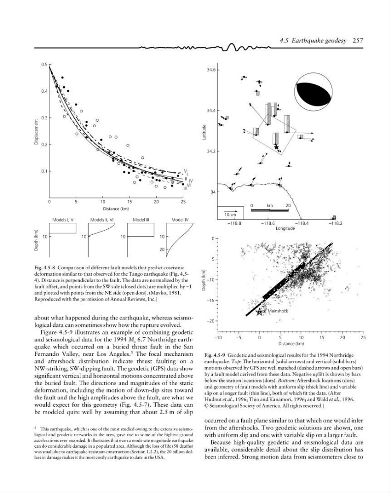
Fig. 4.5-8 Comparison of different fault models that predict coseismic
deformation similar to that observed for the Tango earthquake (Fig. 4.54). Distance is perpendicular to the fault. The data are normalized by the
fault offset, and points from the SW side (closed dots) are multiplied by −1
and plotted with points from the NE side (open dots). (Mavko, 1981.
Reproduced with the permission of Annual Reviews, Inc.)
5 This earthquake, which is one of the most studied owing to the extensive seismological and geodetic networks in the area, gave rise to some of the highest ground
accelerations ever recorded. It illustrates that even a moderate magnitude earthquake
can do considerable damage in a populated area. Although the loss of life (58 deaths)
was small due to earthquake-resistant construction (Section 1.2.2), the 20 billion dollars in damage makes it the most costly earthquake to date in the USA.
about what happened during the earthquake, whereas seismological data can sometimes show how the rupture evolved.
Figure 4.5-9 illustrates an example of combining geodetic
and seismological data for the 1994 M s 6.7 Northridge earthquake which occurred on a buried thrust fault in the San
Fernando Valley, near Los Angeles. 5 The focal mechanism
and aftershock distribution indicate thrust faulting on a
NW-striking, SW-dipping fault. The geodetic (GPS) data show
significant vertical and horizontal motions concentrated above
the buried fault. The directions and magnitudes of the static
deformation, including the motion of down-dip sites toward
the fault and the high amplitudes above the fault, are what we
would expect for this geometry (Fig. 4.5-7). These data can
be modeled quite well by assuming that about 2.5 m of slip
Fig. 4.5-9 Geodetic and seismological results for the 1994 Northridge
earthquake. Top: The horizontal (solid arrows) and vertical (solid bars)
motions observed by GPS are well matched (dashed arrows and open bars)
by a fault model derived from these data. Negative uplift is shown by bars
below the station locations (dots). Bottom: Aftershock locations (dots)
and geometry of fault models with uniform slip (thick line) and variable
slip on a longer fault (thin line), both of which fit the data. (After
Hudnut et al., 1996; Thio and Kanamori, 1996; and Wald et al., 1996.
© Seismological Society of America. All rights reserved.)
occurred on a fault plane similar to that which one would infer
from the aftershocks. Two geodetic solutions are shown, one
with uniform slip and one with variable slip on a larger fault.
Because high-quality geodetic and seismological data are
available, considerable detail about the slip distribution has
been inferred. Strong motion data from seismometers close to
5
−10
−15
−20
25
−10
−5
5
0
1 0
1 5
2 0
Mainshock
Distance (km)
Depth (km)
34.6
34.4
34.2
34
0
k m
2 0
10 cm
−118.8
−118.6
−118.4
−118.2
Longitude
Latitude
4.5 Earthquake geodesy 257
Displacement
0.5
0.4
0.3
0.2
0.1
V
I
II IV
VI
III
0
5
10
15
20
25
Distance (km)
Models I, V
10
Depth (km)
Models II, VI
10
Model III
10
Model IV
10
20
Fig. 4.5-8 Comparison of different fault models that predict coseismic
deformation similar to that observed for the Tango earthquake (Fig. 4.54). Distance is perpendicular to the fault. The data are normalized by the
fault offset, and points from the SW side (closed dots) are multiplied by −1
and plotted with points from the NE side (open dots). (Mavko, 1981.
Reproduced with the permission of Annual Reviews, Inc.)
5 This earthquake, which is one of the most studied owing to the extensive seismological and geodetic networks in the area, gave rise to some of the highest ground
accelerations ever recorded. It illustrates that even a moderate magnitude earthquake
can do considerable damage in a populated area. Although the loss of life (58 deaths)
was small due to earthquake-resistant construction (Section 1.2.2), the 20 billion dollars in damage makes it the most costly earthquake to date in the USA.
about what happened during the earthquake, whereas seismological data can sometimes show how the rupture evolved.
Figure 4.5-9 illustrates an example of combining geodetic
and seismological data for the 1994 M s 6.7 Northridge earthquake which occurred on a buried thrust fault in the San
Fernando Valley, near Los Angeles. 5 The focal mechanism
and aftershock distribution indicate thrust faulting on a
NW-striking, SW-dipping fault. The geodetic (GPS) data show
significant vertical and horizontal motions concentrated above
the buried fault. The directions and magnitudes of the static
deformation, including the motion of down-dip sites toward
the fault and the high amplitudes above the fault, are what we
would expect for this geometry (Fig. 4.5-7). These data can
be modeled quite well by assuming that about 2.5 m of slip
Fig. 4.5-9 Geodetic and seismological results for the 1994 Northridge
earthquake. Top: The horizontal (solid arrows) and vertical (solid bars)
motions observed by GPS are well matched (dashed arrows and open bars)
by a fault model derived from these data. Negative uplift is shown by bars
below the station locations (dots). Bottom: Aftershock locations (dots)
and geometry of fault models with uniform slip (thick line) and variable
slip on a longer fault (thin line), both of which fit the data. (After
Hudnut et al., 1996; Thio and Kanamori, 1996; and Wald et al., 1996.
© Seismological Society of America. All rights reserved.)
occurred on a fault plane similar to that which one would infer
from the aftershocks. Two geodetic solutions are shown, one
with uniform slip and one with variable slip on a larger fault.
Because high-quality geodetic and seismological data are
available, considerable detail about the slip distribution has
been inferred. Strong motion data from seismometers close to