

256 Earthquakes
areas. For a fault that does not reach the surface, the displacement is both reduced in amplitude and varies more smoothly
with distance than it would for a fault extending to the surface.
Such buried dip-slip faults are sometimes called “blind” faults,
because they do not appear at the surface and may not be
recognized until an earthquake occurs.
The general solutions allow modeling of all three components of static displacement for earthquakes with any focal
mechanism and finite fault dimensions. We can also model
situations in which different parts of the fault slip by different
amounts.
Estimating fault parameters from geodetic data is a classic
example of an inverse problem with a highly non-unique
solution, because various combinations of fault parameters
predict similar deformation. Figure 4.5-8 shows six solutions
that all give reasonable fits to the Tango earthquake data
(Fig. 4.5-4). Model I is an infinite fault with uniform slip at
depth, model II is an infinite fault with slip tapering to zero at
depth, and models III and IV are finite faults with uniform and
variable slip, respectively. Model V is the most complicated,
in that it assumes that the material near the fault is weaker
than that further away.
4.5.3 Joint geodetic and seismological earthquake studies
Combining geodetic and seismic wave observations gives more
information than either data type alone. The two data types are
nicely complementary. For example, although seismic waves
have an ambiguity in distinguishing between the fault plane
and the auxiliary plane, the geodetic data do not, as shown by
the fact that the Tango earthquake data (Fig. 4.5-4) and static
displacement models (Fig. 4.5-6, top) do not have a nodal plane
perpendicular to the fault plane. Both data types can give good
constraints on the fault geometry and slip on it, and aftershock
locations often provide the best constraint on fault dimensions.
However, geodetic data that depend on the difference in position before and after an earthquake provide no information
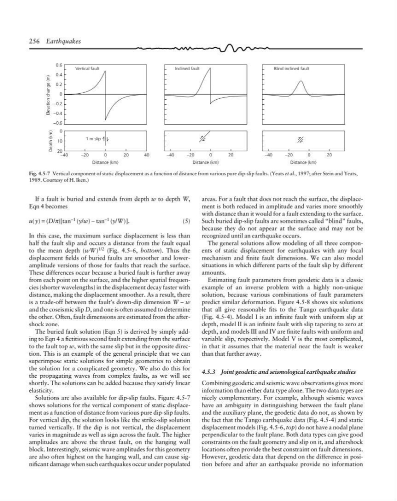
Fig. 4.5-7 Vertical component of static displacement as a function of distance from various pure dip-slip faults. (Yeats et al., 1997; after Stein and Yeats,
1989. Courtesy of H. Iken.)
If a fault is buried and extends from depth w to depth W,
Eqn 4 becomes
u( y) = (D/π)[tan −1 (y/w) − tan −1 (y/W)].
(5)
In this case, the maximum surface displacement is less than
half the fault slip and occurs a distance from the fault equal
to the mean depth (wW ) 1/2 (Fig. 4.5-6, bottom). Thus the
displacement fields of buried faults are smoother and loweramplitude versions of those for faults that reach the surface.
These differences occur because a buried fault is further away
from each point on the surface, and the higher spatial frequencies (shorter wavelengths) in the displacement decay faster with
distance, making the displacement smoother. As a result, there
is a trade-off between the fault’s down-dip dimension W – w
and the coseismic slip D, and one is often assumed to determine
the other. Often, fault dimensions are estimated from the aftershock zone.
The buried fault solution (Eqn 5) is derived by simply adding to Eqn 4 a fictitious second fault extending from the surface
to the fault top w, with the same slip but in the opposite direction. This is an example of the general principle that we can
superimpose static solutions for simple geometries to obtain
the solution for a complicated geometry. We also do this for
the propagating waves from complex faults, as we will see
shortly. The solutions can be added because they satisfy linear
elasticity.
Solutions are also available for dip-slip faults. Figure 4.5-7
shows solutions for the vertical component of static displacement as a function of distance from various pure dip-slip faults.
For vertical dip, the solution looks like the strike-slip solution
turned vertically. If the dip is not vertical, the displacement
varies in magnitude as well as sign across the fault. The higher
amplitudes are above the thrust fault, on the hanging wall
block. Interestingly, seismic wave amplitudes for this geometry
are also often highest on the hanging wall, and can cause significant damage when such earthquakes occur under populated
0.6
0.4
0.2
0
−0.2
−0.4
−0.6
Elevation change (m)
Vertical fault
Inclined fault
Blind inclined fault
Depth (km)
0
10
20
−40
−20
0
20
40
−40
−20
0
20
−40
−20
0
20
1 m slip
Distance (km)
Distance (km)
Distance (km)
areas. For a fault that does not reach the surface, the displacement is both reduced in amplitude and varies more smoothly
with distance than it would for a fault extending to the surface.
Such buried dip-slip faults are sometimes called “blind” faults,
because they do not appear at the surface and may not be
recognized until an earthquake occurs.
The general solutions allow modeling of all three components of static displacement for earthquakes with any focal
mechanism and finite fault dimensions. We can also model
situations in which different parts of the fault slip by different
amounts.
Estimating fault parameters from geodetic data is a classic
example of an inverse problem with a highly non-unique
solution, because various combinations of fault parameters
predict similar deformation. Figure 4.5-8 shows six solutions
that all give reasonable fits to the Tango earthquake data
(Fig. 4.5-4). Model I is an infinite fault with uniform slip at
depth, model II is an infinite fault with slip tapering to zero at
depth, and models III and IV are finite faults with uniform and
variable slip, respectively. Model V is the most complicated,
in that it assumes that the material near the fault is weaker
than that further away.
4.5.3 Joint geodetic and seismological earthquake studies
Combining geodetic and seismic wave observations gives more
information than either data type alone. The two data types are
nicely complementary. For example, although seismic waves
have an ambiguity in distinguishing between the fault plane
and the auxiliary plane, the geodetic data do not, as shown by
the fact that the Tango earthquake data (Fig. 4.5-4) and static
displacement models (Fig. 4.5-6, top) do not have a nodal plane
perpendicular to the fault plane. Both data types can give good
constraints on the fault geometry and slip on it, and aftershock
locations often provide the best constraint on fault dimensions.
However, geodetic data that depend on the difference in position before and after an earthquake provide no information
Fig. 4.5-7 Vertical component of static displacement as a function of distance from various pure dip-slip faults. (Yeats et al., 1997; after Stein and Yeats,
1989. Courtesy of H. Iken.)
If a fault is buried and extends from depth w to depth W,
Eqn 4 becomes
u( y) = (D/π)[tan −1 (y/w) − tan −1 (y/W)].
(5)
In this case, the maximum surface displacement is less than
half the fault slip and occurs a distance from the fault equal
to the mean depth (wW ) 1/2 (Fig. 4.5-6, bottom). Thus the
displacement fields of buried faults are smoother and loweramplitude versions of those for faults that reach the surface.
These differences occur because a buried fault is further away
from each point on the surface, and the higher spatial frequencies (shorter wavelengths) in the displacement decay faster with
distance, making the displacement smoother. As a result, there
is a trade-off between the fault’s down-dip dimension W – w
and the coseismic slip D, and one is often assumed to determine
the other. Often, fault dimensions are estimated from the aftershock zone.
The buried fault solution (Eqn 5) is derived by simply adding to Eqn 4 a fictitious second fault extending from the surface
to the fault top w, with the same slip but in the opposite direction. This is an example of the general principle that we can
superimpose static solutions for simple geometries to obtain
the solution for a complicated geometry. We also do this for
the propagating waves from complex faults, as we will see
shortly. The solutions can be added because they satisfy linear
elasticity.
Solutions are also available for dip-slip faults. Figure 4.5-7
shows solutions for the vertical component of static displacement as a function of distance from various pure dip-slip faults.
For vertical dip, the solution looks like the strike-slip solution
turned vertically. If the dip is not vertical, the displacement
varies in magnitude as well as sign across the fault. The higher
amplitudes are above the thrust fault, on the hanging wall
block. Interestingly, seismic wave amplitudes for this geometry
are also often highest on the hanging wall, and can cause significant damage when such earthquakes occur under populated
0.6
0.4
0.2
0
−0.2
−0.4
−0.6
Elevation change (m)
Vertical fault
Inclined fault
Blind inclined fault
Depth (km)
0
10
20
−40
−20
0
20
40
−40
−20
0
20
−40
−20
0
20
1 m slip
Distance (km)
Distance (km)
Distance (km)