

250 Earthquakes
4 2 is the T axis, and 4 3 is the null axis. Using these axes and our
tectonic preconceptions (which are not, of course, always
valid), we decide (using a stereonet or a computer) that the
earthquake was a thrust on a fault plane striking N189°E
and dipping 23°W. The auxiliary plane strikes N3°E and
dips 67°E.
In this case, we discarded the minor double couple and
assumed that the earthquake was a single double couple. It is
likely that the minor double couple often results from lateral
heterogeneity in the earth (the velocity and attenuation models
used in this inversion were laterally homogeneous), noise in
the data, and deviation of the earthquake from a point source.
You may recall from the surface wave example in Fig. 4.3-13
that the data were approximately fit by the amplitude radiation
pattern predicted by the focal mechanism, but some stations
had higher amplitudes, whereas others had lower amplitudes.
Similar effects can occur for the amplitude and phase data in a
moment tensor inversion. As a result, even if the source were a
pure double couple, the inversion fits the deviations in the data
from the predictions of the best-fitting double couple, and so
yields a moment tensor differing somewhat from the double
couple. Thus the better the inversion method reflects the earth’s
heterogeneity and source complexity, the less the tendency for
there to be spurious portions of the moment tensor. In some
cases, however, the minor double couple may have physical
significance, such as for simultaneous ruptures on nearby faults
with different orientations.
The moment tensor can be decomposed in other ways. One
is into a double couple and a CLVD:
′
′
′
⎛
⎝
⎜
⎜
⎜
⎞
⎠
⎟
⎟
⎟
=
′ + ′
− ′ − ′
⎛
⎝
⎜
⎜
⎜
⎞
⎠
⎟
⎟
⎟
λ
λ
λ
λ
λ
λ
λ
1
2
3
1
3
1
3
0 0
0
0
0 0
2
0
0
0
2 0
0
0
0
/
/
+
− ′
− ′
′
⎛
⎝
⎜
⎜
⎜
⎞
⎠
⎟
⎟
⎟
/
/
.
λ
λ
λ
3
3
3
2
0
0
0
2 0
0
0
(48)
The relative strength of the double couple and CLVD is given
by the ratio of the smallest and largest deviatoric eigenvalues,
ε = λ ′ 3 /λ ′
1 . ε = 0 indicates a pure double couple, and ε = ±0.5
shows a pure CLVD source. About 4% percent of the mechanisms in the Harvard global moment tensor catalog, derived
from inversions that are not constrained to yield double
couples, have | ε | ≥ 0.3. Some of these may be artifacts of the
inversion process similar to spurious minor double couples,
but some appear to be real source effects.
However, as our CLVD example (Section 4.4.6) showed,
both moment tensor decompositions and their interpretations
are not unique. For example, Eqn 45 showed a decomposition into a major double couple with moment λ ′
1 and a minor
double couple with moment λ ′ 3 . We could also decompose the
tensor with the same major double couple but a minor double
couple with moment λ ′ 2 :
5 This example was provided by A. Michael.
λ
λ
λ
λ
λ
λ
1
2
3
1
2
3
0 0
0
0
0 0
0 0
0
0
0 0
0 0
0
0
0 0
⎛
⎝
⎜
⎜
⎜
⎞
⎠
⎟
⎟
⎟
=
⎛
⎝
⎜
⎜
⎜
⎞
⎠
⎟
⎟
⎟
+
′
′
′
⎛
⎝
⎜
⎜
⎜
⎞
⎠
⎟
⎟
⎟
,
E
E
E
(44)
where E = (λ 1 + λ 2 + λ 3 )/3. The remaining term is a deviatoric
moment tensor, with zero isotropic component and components equal to the deviatoric eigenvalues λ′ 1 = λ 1 − E, λ ′ 2 = λ 2 − E,
and λ ′
3 = λ 3 − E. If needed, the deviatoric eigenvalues are
renumbered so that | λ′ 1 | ≥ | λ ′
2 | ≥ | λ′ 3 |. If the inversion has no
isotropic component, the deviatoric moment tensor is the
moment tensor resulting from the inversion.
The deviatoric moment tensor can be decomposed in several
ways. One is in terms of two double couples, called the major
and minor double couples:
′
′
′
⎛
⎝
⎜
⎜
⎜
⎞
⎠
⎟
⎟
⎟
=
′
− ′
⎛
⎝
⎜
⎜
⎜
⎞
⎠
⎟
⎟
⎟
+
− ′
′
⎛
⎝
⎜
⎜
⎜
⎞
⎠
⎟
⎟
⎟
λ
λ
λ
λ
λ
λ
λ
1
2
3
1
1
3
3
0 0
0
0
0 0
0 0
0
0
0
0 0
0 0
0
0
0
0 0
.
(45)
The first tensor is the major double couple, with scalar moment
| λ ′
1 |, and the second is the minor double couple, with scalar
moment | λ ′ 3 |. Usually, the magnitude of the major double
couple is much larger, and we treat it as the earthquake’s
source mechanism.
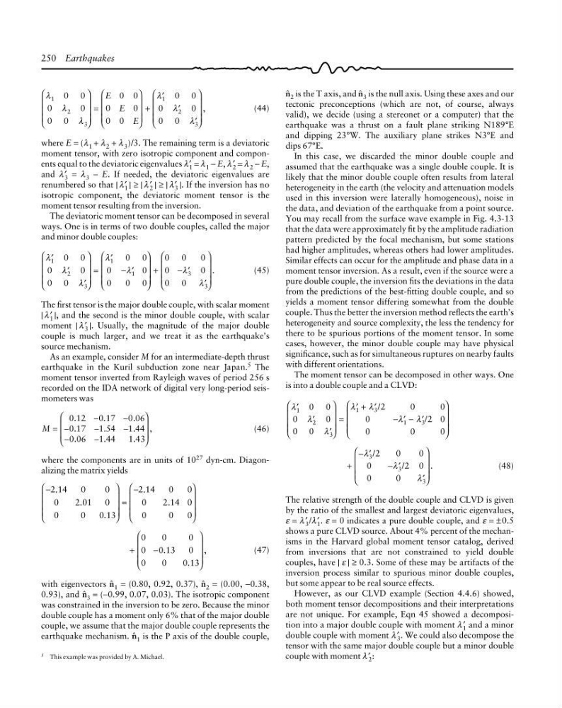
As an example, consider M for an intermediate-depth thrust
earthquake in the Kuril subduction zone near Japan.
5 The
moment tensor inverted from Rayleigh waves of period 256 s
recorded on the IDA network of digital very long-period seismometers was
M
.
.
.
.
.
.
.
.
.
,
=
−
−
−
−
−
−
−
⎛
⎝
⎜
⎜
⎞
⎠
⎟
⎟
0 12 0 17 0 06
0 17
1 54 1 44
0 06 1 44 1 43
(46)
where the components are in units of 10
27 dyn-cm. Diagonalizing the matrix yields
−
⎛
⎝
⎜
⎜
⎜
⎞
⎠
⎟
⎟
⎟
=
−
⎛
⎝
⎜
⎜
⎜
⎞
⎠
⎟
⎟
⎟
2 14
0
0
0
2 01 0
0
0
013
2 14
0
0
0
2 14 0
0
0
0
.
.
.
.
.
+
−
⎛
⎝
⎜
⎜
⎜
⎞
⎠
⎟
⎟
⎟
0
0
0
0 0 13
0
0
0
013
.
.
,
(47)
with eigenvectors 4 1 = (0.80, 0.92, 0.37), 4 2 = (0.00, −0.38,
0.93), and 4 3 = (−0.99, 0.07, 0.03). The isotropic component
was constrained in the inversion to be zero. Because the minor
double couple has a moment only 6% that of the major double
couple, we assume that the major double couple represents the
earthquake mechanism. 4 1 is the P axis of the double couple,
4 2 is the T axis, and 4 3 is the null axis. Using these axes and our
tectonic preconceptions (which are not, of course, always
valid), we decide (using a stereonet or a computer) that the
earthquake was a thrust on a fault plane striking N189°E
and dipping 23°W. The auxiliary plane strikes N3°E and
dips 67°E.
In this case, we discarded the minor double couple and
assumed that the earthquake was a single double couple. It is
likely that the minor double couple often results from lateral
heterogeneity in the earth (the velocity and attenuation models
used in this inversion were laterally homogeneous), noise in
the data, and deviation of the earthquake from a point source.
You may recall from the surface wave example in Fig. 4.3-13
that the data were approximately fit by the amplitude radiation
pattern predicted by the focal mechanism, but some stations
had higher amplitudes, whereas others had lower amplitudes.
Similar effects can occur for the amplitude and phase data in a
moment tensor inversion. As a result, even if the source were a
pure double couple, the inversion fits the deviations in the data
from the predictions of the best-fitting double couple, and so
yields a moment tensor differing somewhat from the double
couple. Thus the better the inversion method reflects the earth’s
heterogeneity and source complexity, the less the tendency for
there to be spurious portions of the moment tensor. In some
cases, however, the minor double couple may have physical
significance, such as for simultaneous ruptures on nearby faults
with different orientations.
The moment tensor can be decomposed in other ways. One
is into a double couple and a CLVD:
′
′
′
⎛
⎝
⎜
⎜
⎜
⎞
⎠
⎟
⎟
⎟
=
′ + ′
− ′ − ′
⎛
⎝
⎜
⎜
⎜
⎞
⎠
⎟
⎟
⎟
λ
λ
λ
λ
λ
λ
λ
1
2
3
1
3
1
3
0 0
0
0
0 0
2
0
0
0
2 0
0
0
0
/
/
+
− ′
− ′
′
⎛
⎝
⎜
⎜
⎜
⎞
⎠
⎟
⎟
⎟
/
/
.
λ
λ
λ
3
3
3
2
0
0
0
2 0
0
0
(48)
The relative strength of the double couple and CLVD is given
by the ratio of the smallest and largest deviatoric eigenvalues,
ε = λ ′ 3 /λ ′
1 . ε = 0 indicates a pure double couple, and ε = ±0.5
shows a pure CLVD source. About 4% percent of the mechanisms in the Harvard global moment tensor catalog, derived
from inversions that are not constrained to yield double
couples, have | ε | ≥ 0.3. Some of these may be artifacts of the
inversion process similar to spurious minor double couples,
but some appear to be real source effects.
However, as our CLVD example (Section 4.4.6) showed,
both moment tensor decompositions and their interpretations
are not unique. For example, Eqn 45 showed a decomposition into a major double couple with moment λ ′
1 and a minor
double couple with moment λ ′ 3 . We could also decompose the
tensor with the same major double couple but a minor double
couple with moment λ ′ 2 :
5 This example was provided by A. Michael.
λ
λ
λ
λ
λ
λ
1
2
3
1
2
3
0 0
0
0
0 0
0 0
0
0
0 0
0 0
0
0
0 0
⎛
⎝
⎜
⎜
⎜
⎞
⎠
⎟
⎟
⎟
=
⎛
⎝
⎜
⎜
⎜
⎞
⎠
⎟
⎟
⎟
+
′
′
′
⎛
⎝
⎜
⎜
⎜
⎞
⎠
⎟
⎟
⎟
,
E
E
E
(44)
where E = (λ 1 + λ 2 + λ 3 )/3. The remaining term is a deviatoric
moment tensor, with zero isotropic component and components equal to the deviatoric eigenvalues λ′ 1 = λ 1 − E, λ ′ 2 = λ 2 − E,
and λ ′
3 = λ 3 − E. If needed, the deviatoric eigenvalues are
renumbered so that | λ′ 1 | ≥ | λ ′
2 | ≥ | λ′ 3 |. If the inversion has no
isotropic component, the deviatoric moment tensor is the
moment tensor resulting from the inversion.
The deviatoric moment tensor can be decomposed in several
ways. One is in terms of two double couples, called the major
and minor double couples:
′
′
′
⎛
⎝
⎜
⎜
⎜
⎞
⎠
⎟
⎟
⎟
=
′
− ′
⎛
⎝
⎜
⎜
⎜
⎞
⎠
⎟
⎟
⎟
+
− ′
′
⎛
⎝
⎜
⎜
⎜
⎞
⎠
⎟
⎟
⎟
λ
λ
λ
λ
λ
λ
λ
1
2
3
1
1
3
3
0 0
0
0
0 0
0 0
0
0
0
0 0
0 0
0
0
0
0 0
.
(45)
The first tensor is the major double couple, with scalar moment
| λ ′
1 |, and the second is the minor double couple, with scalar
moment | λ ′ 3 |. Usually, the magnitude of the major double
couple is much larger, and we treat it as the earthquake’s
source mechanism.
As an example, consider M for an intermediate-depth thrust
earthquake in the Kuril subduction zone near Japan.
5 The
moment tensor inverted from Rayleigh waves of period 256 s
recorded on the IDA network of digital very long-period seismometers was
M
.
.
.
.
.
.
.
.
.
,
=
−
−
−
−
−
−
−
⎛
⎝
⎜
⎜
⎞
⎠
⎟
⎟
0 12 0 17 0 06
0 17
1 54 1 44
0 06 1 44 1 43
(46)
where the components are in units of 10
27 dyn-cm. Diagonalizing the matrix yields
−
⎛
⎝
⎜
⎜
⎜
⎞
⎠
⎟
⎟
⎟
=
−
⎛
⎝
⎜
⎜
⎜
⎞
⎠
⎟
⎟
⎟
2 14
0
0
0
2 01 0
0
0
013
2 14
0
0
0
2 14 0
0
0
0
.
.
.
.
.
+
−
⎛
⎝
⎜
⎜
⎜
⎞
⎠
⎟
⎟
⎟
0
0
0
0 0 13
0
0
0
013
.
.
,
(47)
with eigenvectors 4 1 = (0.80, 0.92, 0.37), 4 2 = (0.00, −0.38,
0.93), and 4 3 = (−0.99, 0.07, 0.03). The isotropic component
was constrained in the inversion to be zero. Because the minor
double couple has a moment only 6% that of the major double
couple, we assume that the major double couple represents the
earthquake mechanism. 4 1 is the P axis of the double couple,