

This problem can be addressed in several ways. One is to
invert shorter-period waves which have larger amplitudes
(Fig. 4.3-14). However, the effects of lateral heterogeneity
increase for shorter periods, due to the shorter wavelengths.
A second approach is to constrain M xz and M yz to be zero and
invert for only the three components M xx , M yy , M xy . This forces
one eigenvector to be vertical and makes the major double
couple take one of three forms: pure strike-slip on a vertical
plane (vertical null axis), thrust faulting on a 45°-dipping plane
(vertical T axis), or normal faulting on a 45°-dipping plane
(vertical P axis). An interesting way to view this is to note
that shallow earthquakes on vertical dip-slip faults, for which
the only nonzero fault geometry factor (Eqn 4.3.20) is q R , have
radiation patterns proportional to Q R (ω) and so excite surface
waves very inefficiently. Hence constraining M xz and M yz to be
zero excludes any vertical dip-slip component from the focal
mechanism, so a complete solution requires other data, such
as first motions or geological knowledge. A third method is to
constrain one nodal plane from first motions and then do a
linear inversion for the second plane.
We can also use this formulation to invert transverse component Love wave data, using the analogous expressions
U(ω, θ, φ) = V(ω, φ)I(ω)
e
i
− π
θ
/
sin
4
e
−iω aθ/c e
−ω aθ/2Qu e
imπ /2
,
(41)
V(ω, φ) =
−
−
⎡
⎣
⎢
⎢
⎤
⎦
⎥
⎥
(
) sin
cos
P
M
M
M
L
x x
y y
x y
1
2
2
2
φ
φ
+
−
+
[
sin
cos ].
iQ M
M
L
x z
y z
φ
φ
(42)
4.4.8 Interpretation of moment tensors
In general, once a moment tensor has been found by inverting
seismograms, it will be more complicated than expected for a
double couple. Even if the source were a pure double couple,
noise in the data and imperfect knowledge of earth structure
would likely produce a tensor that, once diagonalized, would
look like
M =
⎛
⎝
⎜
⎜ ⎜
⎞
⎠
⎟
⎟ ⎟
λ
λ
λ
1
2
3
0 0
0
0
0 0
| λ 1 | ≥ | λ 2 | ≥ | λ 3 |,
(43)
with eigenvectors 4 1 , 4 2 , and 4 3 .
If M represents a double couple, then λ 1 = −λ 2 , and λ 3 = 0.
However, unless the moment tensor was constrained to satisfy
these conditions, it generally will not do so. In most cases,
λ 1 ≈ −λ 2 , and | λ 2 | >> | λ 3 |, so M is approximately, but not
exactly, a double couple. In this case, we interpret the moment
tensor by decomposing it, as we did for the CLVD examples in
Section 4.4.6. If there is an isotropic component, we remove
it via
4.4 Moment tensors 249
V r (ω, φ) = −
−
−
⎡
⎣
⎢
⎢
⎤
⎦
⎥
⎥
sin
(
) cos
P M
M
M
R
x y
y y
x x
2
1
2
2
φ
φ
−
+
+
+
1
2
S M
M
iQ M
M
R
y y
x x
R
y z
x z
(
)
(
sin
cos ),
φ
φ
(37)
so the inversion is for a vector with five components. N R , the
excitation function for an isotropic source, no longer enters
into the radiation pattern.
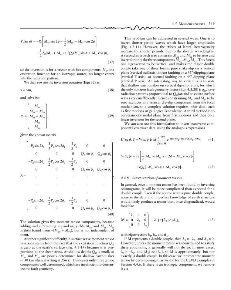
We then rewrite the inversion equation (Eqn 32) as
v = Am,
(38)
and solve for
m
,
=
−
+
⎛
⎝
⎜
⎜
⎜
⎜
⎜
⎜
⎞
⎠
⎟
⎟
⎟
⎟
⎟
⎟
M
M
M
M
M
M
M
xy
yy
xx
yy
xx
yz
xz
(39)
given the known matrix
A
P
P
S
Q
Q
P
P
S
Q
Q
P
P
S
Q
R
R
R
R
R
R
R
R
R
R
R
n
R
n
R
R
=
−
−
−
−
⋅
⋅
⋅
⋅
⋅
⋅
⋅
⋅
⋅
⋅
⋅
⋅
⋅
⋅
⋅
−
−
sin
cos
sin
cos
sin
cos
sin
cos
sin
cos
sin
2
1
2
2
1
2
0
0
0
0
0
2
1
2
2
1
2
0
0
0
0
0
2
1
2
2
1
2
0
0
0
0
0
1
1
1
1
2
2
2
2
φ
φ
φ
φ
φ
φ
φ
φ
φ
φ
φ φ
φ
n
R
n
Q cos
.
⎛
⎝
⎜
⎜
⎜
⎜
⎜
⎜
⎜
⎜
⎜
⎜
⎜
⎜
⎜
⎜
⎜
⎜
⎜
⎜
⎜
⎞
⎠
⎟
⎟
⎟
⎟
⎟
⎟
⎟
⎟
⎟
⎟
⎟
⎟
⎟
⎟
⎟
⎟
⎟
⎟
⎟
(40)
The solution gives five moment tensor components, because
adding and subtracting m 2 and m 3 yields M xx and M yy . M zz
is then found from −(M xx + M yy ), but is not independent of
them.
Another significant difficulty in surface wave moment tensor
inversion stems from the fact that the excitation function Q R
is zero at the earth’s surface (Fig. 4.3-14) because it is proportional to the shear stress. At shallow depths Q R is small, so
M xz and M yz are poorly determined for shallow earthquakes
(< 30 km when inverting at 256 s). This leaves only three tensor
components well determined, which are insufficient to determine the fault geometry.
invert shorter-period waves which have larger amplitudes
(Fig. 4.3-14). However, the effects of lateral heterogeneity
increase for shorter periods, due to the shorter wavelengths.
A second approach is to constrain M xz and M yz to be zero and
invert for only the three components M xx , M yy , M xy . This forces
one eigenvector to be vertical and makes the major double
couple take one of three forms: pure strike-slip on a vertical
plane (vertical null axis), thrust faulting on a 45°-dipping plane
(vertical T axis), or normal faulting on a 45°-dipping plane
(vertical P axis). An interesting way to view this is to note
that shallow earthquakes on vertical dip-slip faults, for which
the only nonzero fault geometry factor (Eqn 4.3.20) is q R , have
radiation patterns proportional to Q R (ω) and so excite surface
waves very inefficiently. Hence constraining M xz and M yz to be
zero excludes any vertical dip-slip component from the focal
mechanism, so a complete solution requires other data, such
as first motions or geological knowledge. A third method is to
constrain one nodal plane from first motions and then do a
linear inversion for the second plane.
We can also use this formulation to invert transverse component Love wave data, using the analogous expressions
U(ω, θ, φ) = V(ω, φ)I(ω)
e
i
− π
θ
/
sin
4
e
−iω aθ/c e
−ω aθ/2Qu e
imπ /2
,
(41)
V(ω, φ) =
−
−
⎡
⎣
⎢
⎢
⎤
⎦
⎥
⎥
(
) sin
cos
P
M
M
M
L
x x
y y
x y
1
2
2
2
φ
φ
+
−
+
[
sin
cos ].
iQ M
M
L
x z
y z
φ
φ
(42)
4.4.8 Interpretation of moment tensors
In general, once a moment tensor has been found by inverting
seismograms, it will be more complicated than expected for a
double couple. Even if the source were a pure double couple,
noise in the data and imperfect knowledge of earth structure
would likely produce a tensor that, once diagonalized, would
look like
M =
⎛
⎝
⎜
⎜ ⎜
⎞
⎠
⎟
⎟ ⎟
λ
λ
λ
1
2
3
0 0
0
0
0 0
| λ 1 | ≥ | λ 2 | ≥ | λ 3 |,
(43)
with eigenvectors 4 1 , 4 2 , and 4 3 .
If M represents a double couple, then λ 1 = −λ 2 , and λ 3 = 0.
However, unless the moment tensor was constrained to satisfy
these conditions, it generally will not do so. In most cases,
λ 1 ≈ −λ 2 , and | λ 2 | >> | λ 3 |, so M is approximately, but not
exactly, a double couple. In this case, we interpret the moment
tensor by decomposing it, as we did for the CLVD examples in
Section 4.4.6. If there is an isotropic component, we remove
it via
4.4 Moment tensors 249
V r (ω, φ) = −
−
−
⎡
⎣
⎢
⎢
⎤
⎦
⎥
⎥
sin
(
) cos
P M
M
M
R
x y
y y
x x
2
1
2
2
φ
φ
−
+
+
+
1
2
S M
M
iQ M
M
R
y y
x x
R
y z
x z
(
)
(
sin
cos ),
φ
φ
(37)
so the inversion is for a vector with five components. N R , the
excitation function for an isotropic source, no longer enters
into the radiation pattern.
We then rewrite the inversion equation (Eqn 32) as
v = Am,
(38)
and solve for
m
,
=
−
+
⎛
⎝
⎜
⎜
⎜
⎜
⎜
⎜
⎞
⎠
⎟
⎟
⎟
⎟
⎟
⎟
M
M
M
M
M
M
M
xy
yy
xx
yy
xx
yz
xz
(39)
given the known matrix
A
P
P
S
Q
Q
P
P
S
Q
Q
P
P
S
Q
R
R
R
R
R
R
R
R
R
R
R
n
R
n
R
R
=
−
−
−
−
⋅
⋅
⋅
⋅
⋅
⋅
⋅
⋅
⋅
⋅
⋅
⋅
⋅
⋅
⋅
−
−
sin
cos
sin
cos
sin
cos
sin
cos
sin
cos
sin
2
1
2
2
1
2
0
0
0
0
0
2
1
2
2
1
2
0
0
0
0
0
2
1
2
2
1
2
0
0
0
0
0
1
1
1
1
2
2
2
2
φ
φ
φ
φ
φ
φ
φ
φ
φ
φ
φ φ
φ
n
R
n
Q cos
.
⎛
⎝
⎜
⎜
⎜
⎜
⎜
⎜
⎜
⎜
⎜
⎜
⎜
⎜
⎜
⎜
⎜
⎜
⎜
⎜
⎜
⎞
⎠
⎟
⎟
⎟
⎟
⎟
⎟
⎟
⎟
⎟
⎟
⎟
⎟
⎟
⎟
⎟
⎟
⎟
⎟
⎟
(40)
The solution gives five moment tensor components, because
adding and subtracting m 2 and m 3 yields M xx and M yy . M zz
is then found from −(M xx + M yy ), but is not independent of
them.
Another significant difficulty in surface wave moment tensor
inversion stems from the fact that the excitation function Q R
is zero at the earth’s surface (Fig. 4.3-14) because it is proportional to the shear stress. At shallow depths Q R is small, so
M xz and M yz are poorly determined for shallow earthquakes
(< 30 km when inverting at 256 s). This leaves only three tensor
components well determined, which are insufficient to determine the fault geometry.