

244 Earthquakes
and recognize that the cross-product of a vector with itself is
zero,
ε ljk d l d k = ε jkl d k d l = 2 × 2 = 0,
ε ljk n l n j = ε klj n l n j = 4 × 4 = 0,
(13)
so the null axis b is an eigenvector with associated eigenvalue 0:
M il b l = 0.
(14)
The fact that the P, T, and null axes are the eigenvectors
of the moment tensor lets us simplify it by transforming it
into the “natural” coordinate system whose basis vectors are
the eigenvectors. Such orthogonal transformations transform a
tensor from one orthogonal coordinate system to another, such
that its components change, but its physical meaning does not.
The transformation matrix with the eigenvectors as columns
(Section A.5.3),
U
t b p
t b p
t b p
,
=
⎛
⎝
⎜
⎜ ⎜
⎞
⎠
⎟
⎟ ⎟
1
1
1
2
2
2
3
3
3
(15)
gives a diagonal moment tensor for a double couple in the
principal axis coordinate system
U
U
M
M
−
=
−
⎛
⎝
⎜
⎜ ⎜
⎞
⎠
⎟
⎟ ⎟
1
0
0
0
0
0 0
0
0 0
M
.
(16)
One diagonal element is zero, and the other two are ± the scalar
moment. The trace (M xx + M yy + M zz ), which is not changed by
an orthogonal transformation, started as zero in Eqn 6 and so
remains zero. Put another way, the isotropic component is an
invariant of the moment tensor and does not depend on the
coordinate system.
The point of the transformation is that inverting seismograms
in a geographic coordinate system yields the moment tensor
in that coordinate system. We then find its eigenvectors, the P,
T, and null axes, and use Eqn 7 to find the fault normal and
slip vectors and hence strike, dip, and slip angles. As part of the
same process, the eigenvalues give the scalar moment.
Thus the moment tensor corresponding to a specific faulting
geometry can be written in different ways. Figure 4.4-1 shows
this in a two-dimensional geometry. The coordinate system oriented along and perpendicular to the fault has the fault normal
and slip vectors as basis vectors, and the nonzero moment
tensor components are M xy = M yx = M 0 (Eqn 3). If we transform
the moment tensor to the new (primed) coordinate system with
the P and T axes as basis vectors, 45° away from the first set, a
two-dimensional version of Eqn 16 gives the moment tensor
M x′x′ = −M y′y′ = M 0 . The transformation changes the components, but the physical moment tensor stays the same, so these
two different-looking force systems give the same radiated
seismic waves. Hence the seismic waves alone provide no way
of deciding which is more “real.” Given that most earthquakes
occur on faults about which we have other knowledge, we generally view earthquakes as slip on a fault rather than dipoles.
It is worth recalling that a similar concept appears whenever
we transform vector or tensor quantities between coordinate
systems. For example, Fig. 2.3-6 showed that a given physical
state of stress could be represented either by normal stresses
(diagonal terms in the stress tensor) or shear stresses (offdiagonal terms in the stress tensor), depending on the coordinate system.
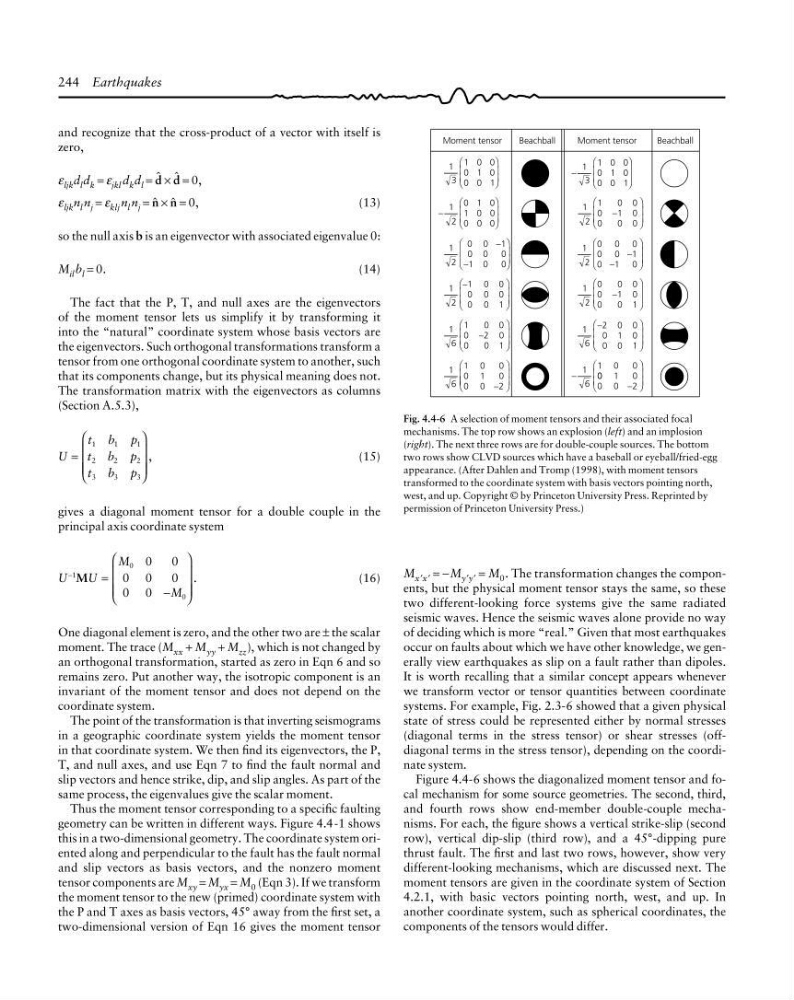
Figure 4.4-6 shows the diagonalized moment tensor and focal mechanism for some source geometries. The second, third,
and fourth rows show end-member double-couple mechanisms. For each, the figure shows a vertical strike-slip (second
row), vertical dip-slip (third row), and a 45°-dipping pure
thrust fault. The first and last two rows, however, show very
different-looking mechanisms, which are discussed next. The
moment tensors are given in the coordinate system of Section
4.2.1, with basic vectors pointing north, west, and up. In
another coordinate system, such as spherical coordinates, the
components of the tensors would differ.
Fig. 4.4-6 A selection of moment tensors and their associated focal
mechanisms. The top row shows an explosion (left) and an implosion
(right). The next three rows are for double-couple sources. The bottom
two rows show CLVD sources which have a baseball or eyeball/fried-egg
appearance. (After Dahlen and Tromp (1998), with moment tensors
transformed to the coordinate system with basis vectors pointing north,
west, and up. Copyright © by Princeton University Press. Reprinted by
permission of Princeton University Press.)
1
3
1 0 0
0 1 0
0 0 1
1
2
0 1 0
1 0 0
0 0 0
1
2
0 0 −1
0 0 0
−1 0 0
1
2
1 0 0
0 0 0
0 0 1
1
6
1
0 0
0 −2 0
0
0 1
1
6
1 0
0
0 1
0
0 0 −2
⎛
⎝
⎜
⎜
⎞
⎠
⎟
⎟
−
⎛
⎝
⎜
⎜
⎞
⎠
⎟
⎟
⎛
⎝
⎜
⎜
⎞
⎠
⎟
⎟
⎛
⎝
⎜
⎜
⎞
⎠
⎟
⎟
⎛
⎝
⎜
⎜
⎞
⎠
⎟
⎟
⎛
⎝
⎜
⎜ ⎜
⎞
⎠
⎟
⎟
−
⎛
⎝
⎜
⎜
⎞
⎠
⎟
⎟
⎛
⎝
⎜
⎜
⎞
⎠
⎟
⎟
⎛
⎝
⎜
⎜
⎞
⎠
⎟
⎟
⎛
⎝
⎜
⎜
⎞
⎠
⎟
⎟
⎛
⎝
⎜
⎜
⎞
⎠
⎟
⎟
−
1
3
1 0 0
0 1 0
0 0 1
1
2
1
0 0
0 −1 0
0
0 0
1
2
0 0 0
0 0 −1
0 −1 0
1
2
0
0 0
0 −1 0
0
0 1
1
6
−2 0 0
0 1 0
0 0 1
1
6
1 0
0
0 0 1
0
0 0 −2
⎛
⎝
⎜
⎜
⎞
⎠
⎟
⎟
Moment tensor
Beachball
Moment tensor
Beachball
−
and recognize that the cross-product of a vector with itself is
zero,
ε ljk d l d k = ε jkl d k d l = 2 × 2 = 0,
ε ljk n l n j = ε klj n l n j = 4 × 4 = 0,
(13)
so the null axis b is an eigenvector with associated eigenvalue 0:
M il b l = 0.
(14)
The fact that the P, T, and null axes are the eigenvectors
of the moment tensor lets us simplify it by transforming it
into the “natural” coordinate system whose basis vectors are
the eigenvectors. Such orthogonal transformations transform a
tensor from one orthogonal coordinate system to another, such
that its components change, but its physical meaning does not.
The transformation matrix with the eigenvectors as columns
(Section A.5.3),
U
t b p
t b p
t b p
,
=
⎛
⎝
⎜
⎜ ⎜
⎞
⎠
⎟
⎟ ⎟
1
1
1
2
2
2
3
3
3
(15)
gives a diagonal moment tensor for a double couple in the
principal axis coordinate system
U
U
M
M
−
=
−
⎛
⎝
⎜
⎜ ⎜
⎞
⎠
⎟
⎟ ⎟
1
0
0
0
0
0 0
0
0 0
M
.
(16)
One diagonal element is zero, and the other two are ± the scalar
moment. The trace (M xx + M yy + M zz ), which is not changed by
an orthogonal transformation, started as zero in Eqn 6 and so
remains zero. Put another way, the isotropic component is an
invariant of the moment tensor and does not depend on the
coordinate system.
The point of the transformation is that inverting seismograms
in a geographic coordinate system yields the moment tensor
in that coordinate system. We then find its eigenvectors, the P,
T, and null axes, and use Eqn 7 to find the fault normal and
slip vectors and hence strike, dip, and slip angles. As part of the
same process, the eigenvalues give the scalar moment.
Thus the moment tensor corresponding to a specific faulting
geometry can be written in different ways. Figure 4.4-1 shows
this in a two-dimensional geometry. The coordinate system oriented along and perpendicular to the fault has the fault normal
and slip vectors as basis vectors, and the nonzero moment
tensor components are M xy = M yx = M 0 (Eqn 3). If we transform
the moment tensor to the new (primed) coordinate system with
the P and T axes as basis vectors, 45° away from the first set, a
two-dimensional version of Eqn 16 gives the moment tensor
M x′x′ = −M y′y′ = M 0 . The transformation changes the components, but the physical moment tensor stays the same, so these
two different-looking force systems give the same radiated
seismic waves. Hence the seismic waves alone provide no way
of deciding which is more “real.” Given that most earthquakes
occur on faults about which we have other knowledge, we generally view earthquakes as slip on a fault rather than dipoles.
It is worth recalling that a similar concept appears whenever
we transform vector or tensor quantities between coordinate
systems. For example, Fig. 2.3-6 showed that a given physical
state of stress could be represented either by normal stresses
(diagonal terms in the stress tensor) or shear stresses (offdiagonal terms in the stress tensor), depending on the coordinate system.
Figure 4.4-6 shows the diagonalized moment tensor and focal mechanism for some source geometries. The second, third,
and fourth rows show end-member double-couple mechanisms. For each, the figure shows a vertical strike-slip (second
row), vertical dip-slip (third row), and a 45°-dipping pure
thrust fault. The first and last two rows, however, show very
different-looking mechanisms, which are discussed next. The
moment tensors are given in the coordinate system of Section
4.2.1, with basic vectors pointing north, west, and up. In
another coordinate system, such as spherical coordinates, the
components of the tensors would differ.
Fig. 4.4-6 A selection of moment tensors and their associated focal
mechanisms. The top row shows an explosion (left) and an implosion
(right). The next three rows are for double-couple sources. The bottom
two rows show CLVD sources which have a baseball or eyeball/fried-egg
appearance. (After Dahlen and Tromp (1998), with moment tensors
transformed to the coordinate system with basis vectors pointing north,
west, and up. Copyright © by Princeton University Press. Reprinted by
permission of Princeton University Press.)
1
3
1 0 0
0 1 0
0 0 1
1
2
0 1 0
1 0 0
0 0 0
1
2
0 0 −1
0 0 0
−1 0 0
1
2
1 0 0
0 0 0
0 0 1
1
6
1
0 0
0 −2 0
0
0 1
1
6
1 0
0
0 1
0
0 0 −2
⎛
⎝
⎜
⎜
⎞
⎠
⎟
⎟
−
⎛
⎝
⎜
⎜
⎞
⎠
⎟
⎟
⎛
⎝
⎜
⎜
⎞
⎠
⎟
⎟
⎛
⎝
⎜
⎜
⎞
⎠
⎟
⎟
⎛
⎝
⎜
⎜
⎞
⎠
⎟
⎟
⎛
⎝
⎜
⎜ ⎜
⎞
⎠
⎟
⎟
−
⎛
⎝
⎜
⎜
⎞
⎠
⎟
⎟
⎛
⎝
⎜
⎜
⎞
⎠
⎟
⎟
⎛
⎝
⎜
⎜
⎞
⎠
⎟
⎟
⎛
⎝
⎜
⎜
⎞
⎠
⎟
⎟
⎛
⎝
⎜
⎜
⎞
⎠
⎟
⎟
−
1
3
1 0 0
0 1 0
0 0 1
1
2
1
0 0
0 −1 0
0
0 0
1
2
0 0 0
0 0 −1
0 −1 0
1
2
0
0 0
0 −1 0
0
0 1
1
6
−2 0 0
0 1 0
0 0 1
1
6
1 0
0
0 0 1
0
0 0 −2
⎛
⎝
⎜
⎜
⎞
⎠
⎟
⎟
Moment tensor
Beachball
Moment tensor
Beachball
−