

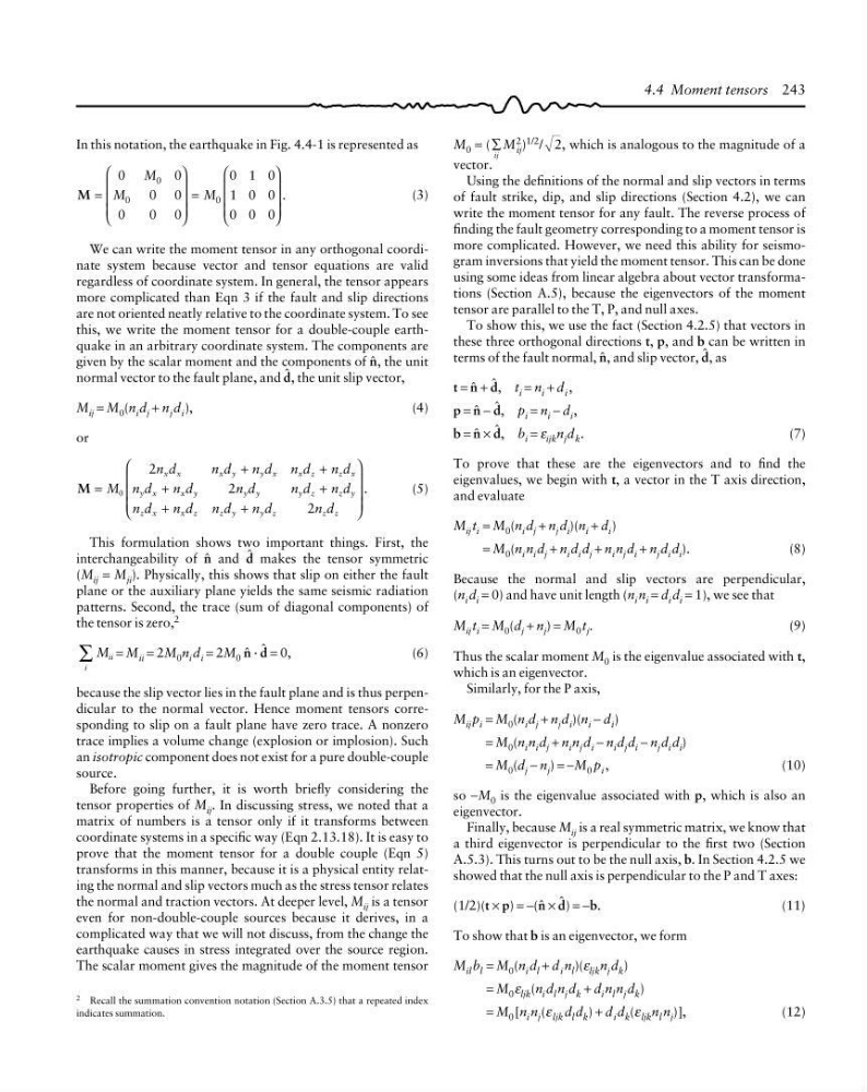
In this notation, the earthquake in Fig. 4.4-1 is represented as
M
.
=
⎛
⎝
⎜
⎜
⎜
⎞
⎠
⎟
⎟
⎟
=
⎛
⎝
⎜
⎜
⎜
⎞
⎠
⎟
⎟
⎟
0
0
0 0
0
0 0
0 1 0
1 0 0
0 0 0
0
0
0
M
M
M
(3)
We can write the moment tensor in any orthogonal coordinate system because vector and tensor equations are valid
regardless of coordinate system. In general, the tensor appears
more complicated than Eqn 3 if the fault and slip directions
are not oriented neatly relative to the coordinate system. To see
this, we write the moment tensor for a double-couple earthquake in an arbitrary coordinate system. The components are
given by the scalar moment and the components of 4, the unit
normal vector to the fault plane, and 2, the unit slip vector,
M ij = M 0 (n i d j + n j d i ),
(4)
or
M
.
=
+
+
+
+
+
+
⎛
⎝
⎜
⎜
⎜
⎞
⎠
⎟
⎟
⎟
M
n d
n d
n d n d
n d
n d
n d
n d
n d
n d
n d
n d n d
n d
n d
x x
x y
y x
x z
z x
y x
x y
y y
y z
z y
z x
x z
z y
y z
z z
0
2
2
2
(5)
This formulation shows two important things. First, the
interchangeability of 4 and 2 makes the tensor symmetric
(M ij = M ji ). Physically, this shows that slip on either the fault
plane or the auxiliary plane yields the same seismic radiation
patterns. Second, the trace (sum of diagonal components) of
the tensor is zero, 2
M ii
i
∑ = M ii = 2M 0 n i d i = 2M 0 4 · 2 = 0,
(6)
because the slip vector lies in the fault plane and is thus perpendicular to the normal vector. Hence moment tensors corresponding to slip on a fault plane have zero trace. A nonzero
trace implies a volume change (explosion or implosion). Such
an isotropic component does not exist for a pure double-couple
source.
Before going further, it is worth briefly considering the
tensor properties of M ij . In discussing stress, we noted that a
matrix of numbers is a tensor only if it transforms between
coordinate systems in a specific way (Eqn 2.13.18). It is easy to
prove that the moment tensor for a double couple (Eqn 5)
transforms in this manner, because it is a physical entity relating the normal and slip vectors much as the stress tensor relates
the normal and traction vectors. At deeper level, M ij is a tensor
even for non-double-couple sources because it derives, in a
complicated way that we will not discuss, from the change the
earthquake causes in stress integrated over the source region.
The scalar moment gives the magnitude of the moment tensor
M 0 = ( ∑
ij
M 2
ij ) 1/2 / 2, which is analogous to the magnitude of a
vector.
Using the definitions of the normal and slip vectors in terms
of fault strike, dip, and slip directions (Section 4.2), we can
write the moment tensor for any fault. The reverse process of
finding the fault geometry corresponding to a moment tensor is
more complicated. However, we need this ability for seismogram inversions that yield the moment tensor. This can be done
using some ideas from linear algebra about vector transformations (Section A.5), because the eigenvectors of the moment
tensor are parallel to the T, P, and null axes.
To show this, we use the fact (Section 4.2.5) that vectors in
these three orthogonal directions t, p, and b can be written in
terms of the fault normal, 4, and slip vector, 2, as
t = 4 + 2, t i = n i + d i ,
p = 4 − 2, p i = n i − d i ,
b = 4 × 2, b i = ε ijk n j d k .
(7)
To prove that these are the eigenvectors and to find the
eigenvalues, we begin with t, a vector in the T axis direction,
and evaluate
M ij t i = M 0 (n i d j + n j d i )(n i + d i )
= M 0 (n i n i d j + n i d i d j + n i n j d i + n j d i d i ).
(8)
Because the normal and slip vectors are perpendicular,
(n i d i = 0) and have unit length (n i n i = d i d i = 1), we see that
M ij t i = M 0 (d j + n j ) = M 0 t j .
(9)
Thus the scalar moment M 0 is the eigenvalue associated with t,
which is an eigenvector.
Similarly, for the P axis,
M ij p i = M 0 (n i d j + n j d i )(n i − d i )
= M 0 (n i n i d j + n i n j d i − n i d j d i − n j d i d i )
= M 0 (d j − n j ) = −M 0 p i ,
(10)
so −M 0 is the eigenvalue associated with p, which is also an
eigenvector.
Finally, because M ij is a real symmetric matrix, we know that
a third eigenvector is perpendicular to the first two (Section
A.5.3). This turns out to be the null axis, b. In Section 4.2.5 we
showed that the null axis is perpendicular to the P and T axes:
(1/2)(t × p) = −(4 × 2) = −b.
(11)
To show that b is an eigenvector, we form
M il b l = M 0 (n i d l + d i n l )(ε ljk n j d k )
= M 0 ε ljk (n i d l n j d k + d i n l n j d k )
= M 0 [n i n j (ε ljk d l d k ) + d i d k (ε ljk n l n j )],
(12)
4.4 Moment tensors 243
2 Recall the summation convention notation (Section A.3.5) that a repeated index
indicates summation.
M
.
=
⎛
⎝
⎜
⎜
⎜
⎞
⎠
⎟
⎟
⎟
=
⎛
⎝
⎜
⎜
⎜
⎞
⎠
⎟
⎟
⎟
0
0
0 0
0
0 0
0 1 0
1 0 0
0 0 0
0
0
0
M
M
M
(3)
We can write the moment tensor in any orthogonal coordinate system because vector and tensor equations are valid
regardless of coordinate system. In general, the tensor appears
more complicated than Eqn 3 if the fault and slip directions
are not oriented neatly relative to the coordinate system. To see
this, we write the moment tensor for a double-couple earthquake in an arbitrary coordinate system. The components are
given by the scalar moment and the components of 4, the unit
normal vector to the fault plane, and 2, the unit slip vector,
M ij = M 0 (n i d j + n j d i ),
(4)
or
M
.
=
+
+
+
+
+
+
⎛
⎝
⎜
⎜
⎜
⎞
⎠
⎟
⎟
⎟
M
n d
n d
n d n d
n d
n d
n d
n d
n d
n d
n d
n d n d
n d
n d
x x
x y
y x
x z
z x
y x
x y
y y
y z
z y
z x
x z
z y
y z
z z
0
2
2
2
(5)
This formulation shows two important things. First, the
interchangeability of 4 and 2 makes the tensor symmetric
(M ij = M ji ). Physically, this shows that slip on either the fault
plane or the auxiliary plane yields the same seismic radiation
patterns. Second, the trace (sum of diagonal components) of
the tensor is zero, 2
M ii
i
∑ = M ii = 2M 0 n i d i = 2M 0 4 · 2 = 0,
(6)
because the slip vector lies in the fault plane and is thus perpendicular to the normal vector. Hence moment tensors corresponding to slip on a fault plane have zero trace. A nonzero
trace implies a volume change (explosion or implosion). Such
an isotropic component does not exist for a pure double-couple
source.
Before going further, it is worth briefly considering the
tensor properties of M ij . In discussing stress, we noted that a
matrix of numbers is a tensor only if it transforms between
coordinate systems in a specific way (Eqn 2.13.18). It is easy to
prove that the moment tensor for a double couple (Eqn 5)
transforms in this manner, because it is a physical entity relating the normal and slip vectors much as the stress tensor relates
the normal and traction vectors. At deeper level, M ij is a tensor
even for non-double-couple sources because it derives, in a
complicated way that we will not discuss, from the change the
earthquake causes in stress integrated over the source region.
The scalar moment gives the magnitude of the moment tensor
M 0 = ( ∑
ij
M 2
ij ) 1/2 / 2, which is analogous to the magnitude of a
vector.
Using the definitions of the normal and slip vectors in terms
of fault strike, dip, and slip directions (Section 4.2), we can
write the moment tensor for any fault. The reverse process of
finding the fault geometry corresponding to a moment tensor is
more complicated. However, we need this ability for seismogram inversions that yield the moment tensor. This can be done
using some ideas from linear algebra about vector transformations (Section A.5), because the eigenvectors of the moment
tensor are parallel to the T, P, and null axes.
To show this, we use the fact (Section 4.2.5) that vectors in
these three orthogonal directions t, p, and b can be written in
terms of the fault normal, 4, and slip vector, 2, as
t = 4 + 2, t i = n i + d i ,
p = 4 − 2, p i = n i − d i ,
b = 4 × 2, b i = ε ijk n j d k .
(7)
To prove that these are the eigenvectors and to find the
eigenvalues, we begin with t, a vector in the T axis direction,
and evaluate
M ij t i = M 0 (n i d j + n j d i )(n i + d i )
= M 0 (n i n i d j + n i d i d j + n i n j d i + n j d i d i ).
(8)
Because the normal and slip vectors are perpendicular,
(n i d i = 0) and have unit length (n i n i = d i d i = 1), we see that
M ij t i = M 0 (d j + n j ) = M 0 t j .
(9)
Thus the scalar moment M 0 is the eigenvalue associated with t,
which is an eigenvector.
Similarly, for the P axis,
M ij p i = M 0 (n i d j + n j d i )(n i − d i )
= M 0 (n i n i d j + n i n j d i − n i d j d i − n j d i d i )
= M 0 (d j − n j ) = −M 0 p i ,
(10)
so −M 0 is the eigenvalue associated with p, which is also an
eigenvector.
Finally, because M ij is a real symmetric matrix, we know that
a third eigenvector is perpendicular to the first two (Section
A.5.3). This turns out to be the null axis, b. In Section 4.2.5 we
showed that the null axis is perpendicular to the P and T axes:
(1/2)(t × p) = −(4 × 2) = −b.
(11)
To show that b is an eigenvector, we form
M il b l = M 0 (n i d l + d i n l )(ε ljk n j d k )
= M 0 ε ljk (n i d l n j d k + d i n l n j d k )
= M 0 [n i n j (ε ljk d l d k ) + d i d k (ε ljk n l n j )],
(12)
4.4 Moment tensors 243
2 Recall the summation convention notation (Section A.3.5) that a repeated index
indicates summation.