

Love
Rayleigh
November 11, 1967
m b = 5.6
M s = 5.2
4.3 Waveform modeling 237
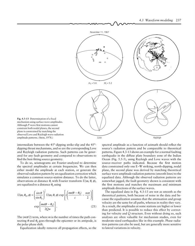
Fig. 4.3-13 Determination of a focal
mechanism using surface wave amplitudes.
Although P-wave first motions cannot
constrain both nodal planes, the second
plane is constrained by matching the
observed Love and Rayleigh wave radiation
amplitude patterns. (Stein, 1978.)
intermediate between the 45°-dipping strike-slip and the 45°dipping thrust mechanisms, and so are the corresponding Love
and Rayleigh radiation patterns. Such patterns can be generated for any fault geometry and compared to observations to
find the best-fitting source geometry.
To do so, seismograms are Fourier-analyzed to determine
the spectral amplitudes at certain frequencies. We can then
either model the amplitude at each station, or generate the
observed radiation pattern by an equalization correction which
simulates a common source-station distance. To do the latter,
observations at distance θ, with Fourier transform U(ω, θ, φ),
are equalized to a distance θ 0 using
U
U
i
a
c
m
( , , )
sin
sin
( , , ) exp
(
)
ω θ φ
θ
θ
ω θ φ
ω θ θ
π
0
0
0
1
2
2
=
⎛
⎝
⎜
⎞
⎠
⎟
−
−
⎛
⎝
⎜
⎞
⎠
⎟
⎡
⎣
⎢
⎢
⎤
⎦
⎥
⎥
exp
(
) .
ω θ θ
a
Qu
−
⎡
⎣
⎢
⎢
⎤
⎦
⎥
⎥
0
2
(21)
The (mπ/2) term, where m is the number of times the path connecting θ and θ 0 goes through the epicenter or its antipode, is
the polar phase shift.
Equalization ideally removes all propagation effects, so the
spectral amplitude as a function of azimuth should reflect the
source’s radiation pattern and be comparable to theoretical
patterns. Figure 4.3-13 shows an example for a normal faulting
earthquake in the diffuse plate boundary zone of the Indian
Ocean (Fig. 5.5-5), using Rayleigh and Love waves with the
source–receiver paths indicated. Because the first motion
data constrained only one E–W striking, north-dipping, nodal
plane, the second plane was derived by matching theoretical
surface wave amplitude radiation patterns (smooth lines) to the
equalized data. Although the observed radiation patterns are
somewhat jagged, the fault geometry shown is consistent with
the first motions and matches the maximum and minimum
amplitude directions of the surface waves.
The equalized data in Fig. 4.3-13 are not as smooth as the
theoretical pattern, both because of noise in the data and because the equalization assumes that the attenuation and group
velocity are the same for all paths, whereas in reality they vary.
As a result, the amplitudes at some stations are higher or lower
than predicted. It is possible to reduce this effect by correcting for velocity and Q structure. Even without doing so, such
analyses are often valuable for mechanism studies, even for
moderate-sized earthquakes like in this example. Phase radiation patterns can also be used, but are generally more sensitive
to lateral variations in velocity.
Rayleigh
November 11, 1967
m b = 5.6
M s = 5.2
4.3 Waveform modeling 237
Fig. 4.3-13 Determination of a focal
mechanism using surface wave amplitudes.
Although P-wave first motions cannot
constrain both nodal planes, the second
plane is constrained by matching the
observed Love and Rayleigh wave radiation
amplitude patterns. (Stein, 1978.)
intermediate between the 45°-dipping strike-slip and the 45°dipping thrust mechanisms, and so are the corresponding Love
and Rayleigh radiation patterns. Such patterns can be generated for any fault geometry and compared to observations to
find the best-fitting source geometry.
To do so, seismograms are Fourier-analyzed to determine
the spectral amplitudes at certain frequencies. We can then
either model the amplitude at each station, or generate the
observed radiation pattern by an equalization correction which
simulates a common source-station distance. To do the latter,
observations at distance θ, with Fourier transform U(ω, θ, φ),
are equalized to a distance θ 0 using
U
U
i
a
c
m
( , , )
sin
sin
( , , ) exp
(
)
ω θ φ
θ
θ
ω θ φ
ω θ θ
π
0
0
0
1
2
2
=
⎛
⎝
⎜
⎞
⎠
⎟
−
−
⎛
⎝
⎜
⎞
⎠
⎟
⎡
⎣
⎢
⎢
⎤
⎦
⎥
⎥
exp
(
) .
ω θ θ
a
Qu
−
⎡
⎣
⎢
⎢
⎤
⎦
⎥
⎥
0
2
(21)
The (mπ/2) term, where m is the number of times the path connecting θ and θ 0 goes through the epicenter or its antipode, is
the polar phase shift.
Equalization ideally removes all propagation effects, so the
spectral amplitude as a function of azimuth should reflect the
source’s radiation pattern and be comparable to theoretical
patterns. Figure 4.3-13 shows an example for a normal faulting
earthquake in the diffuse plate boundary zone of the Indian
Ocean (Fig. 5.5-5), using Rayleigh and Love waves with the
source–receiver paths indicated. Because the first motion
data constrained only one E–W striking, north-dipping, nodal
plane, the second plane was derived by matching theoretical
surface wave amplitude radiation patterns (smooth lines) to the
equalized data. Although the observed radiation patterns are
somewhat jagged, the fault geometry shown is consistent with
the first motions and matches the maximum and minimum
amplitude directions of the surface waves.
The equalized data in Fig. 4.3-13 are not as smooth as the
theoretical pattern, both because of noise in the data and because the equalization assumes that the attenuation and group
velocity are the same for all paths, whereas in reality they vary.
As a result, the amplitudes at some stations are higher or lower
than predicted. It is possible to reduce this effect by correcting for velocity and Q structure. Even without doing so, such
analyses are often valuable for mechanism studies, even for
moderate-sized earthquakes like in this example. Phase radiation patterns can also be used, but are generally more sensitive
to lateral variations in velocity.