

238 Earthquakes
S R (w)
5
4
3
2
1
0
320 213 160 128
h = 0.
h = 11.
h = 37.
h = 62.
h = 88.
h = 116.
Period (s)
256
142
256 196 142
320 213 160 128
P R (w)
h = 0.
h = 11.
h = 37.
h = 62.
h = 88.
h = 116.
h = 214.
Period (s)
256 196 142
320 213 160 128
Q R (w)
h = 0.
h = 11.
h = 37.
h = 62.
h = 88.
h = 116.
Period (s)
0.5
0
–0.5
3
2
1
0
0
4
5
6
10
30
40
50
20
Period (s)
10
–3
Amplitude (cm-s)
ω
ω
ω
Surface waves can also be used to study fault length and rupture for large earthquakes. Figure 4.3-15 shows an analysis for
the great 1964 Alaska earthquake, the second largest ever
instrumentally recorded (Fig. 1.2-2). The focal mechanism
and geodetic data imply thrust faulting on a roughly NE–SWstriking, shallow NW-dipping fault, due to the subduction of
the Pacific plate beneath North America (Fig. 5.2-3). The earthquake was so large that surface waves were unusable until their
amplitude had decayed enough, by the fifth station passage (R5
and G5, Fig. 2.7-3). From Fig. 4.3-12, we would expect both
the Love and Rayleigh wave amplitude radiation patterns to
have minima in the strike direction. However, the observed
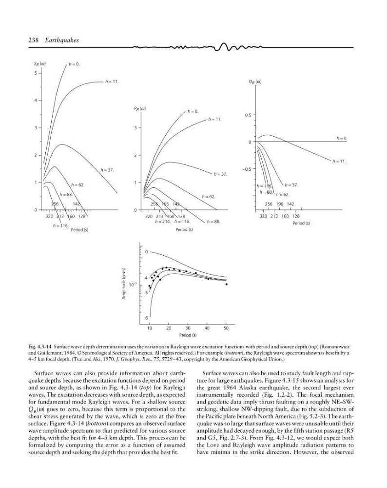
Surface waves can also provide information about earthquake depths because the excitation functions depend on period
and source depth, as shown in Fig. 4.3-14 (top) for Rayleigh
waves. The excitation decreases with source depth, as expected
for fundamental mode Rayleigh waves. For a shallow source
Q R (ω) goes to zero, because this term is proportional to the
shear stress generated by the wave, which is zero at the free
surface. Figure 4.3-14 (bottom) compares an observed surface
wave amplitude spectrum to that predicted for various source
depths, with the best fit for 4–5 km depth. This process can be
formalized by computing the error as a function of assumed
source depth and seeking the depth that provides the best fit.
Fig. 4.3-14 Surface wave depth determination uses the variation in Rayleigh wave excitation functions with period and source depth (top) (Romanowicz
and Guillemant, 1984. © Seismological Society of America. All rights reserved.) For example (bottom), the Rayleigh wave spectrum shown is best fit by a
4–5 km focal depth. (Tsai and Aki, 1970. J. Geophys. Res., 75, 5729–43, copyright by the American Geophysical Union.)
S R (w)
5
4
3
2
1
0
320 213 160 128
h = 0.
h = 11.
h = 37.
h = 62.
h = 88.
h = 116.
Period (s)
256
142
256 196 142
320 213 160 128
P R (w)
h = 0.
h = 11.
h = 37.
h = 62.
h = 88.
h = 116.
h = 214.
Period (s)
256 196 142
320 213 160 128
Q R (w)
h = 0.
h = 11.
h = 37.
h = 62.
h = 88.
h = 116.
Period (s)
0.5
0
–0.5
3
2
1
0
0
4
5
6
10
30
40
50
20
Period (s)
10
–3
Amplitude (cm-s)
ω
ω
ω
Surface waves can also be used to study fault length and rupture for large earthquakes. Figure 4.3-15 shows an analysis for
the great 1964 Alaska earthquake, the second largest ever
instrumentally recorded (Fig. 1.2-2). The focal mechanism
and geodetic data imply thrust faulting on a roughly NE–SWstriking, shallow NW-dipping fault, due to the subduction of
the Pacific plate beneath North America (Fig. 5.2-3). The earthquake was so large that surface waves were unusable until their
amplitude had decayed enough, by the fifth station passage (R5
and G5, Fig. 2.7-3). From Fig. 4.3-12, we would expect both
the Love and Rayleigh wave amplitude radiation patterns to
have minima in the strike direction. However, the observed
Surface waves can also provide information about earthquake depths because the excitation functions depend on period
and source depth, as shown in Fig. 4.3-14 (top) for Rayleigh
waves. The excitation decreases with source depth, as expected
for fundamental mode Rayleigh waves. For a shallow source
Q R (ω) goes to zero, because this term is proportional to the
shear stress generated by the wave, which is zero at the free
surface. Figure 4.3-14 (bottom) compares an observed surface
wave amplitude spectrum to that predicted for various source
depths, with the best fit for 4–5 km depth. This process can be
formalized by computing the error as a function of assumed
source depth and seeking the depth that provides the best fit.
Fig. 4.3-14 Surface wave depth determination uses the variation in Rayleigh wave excitation functions with period and source depth (top) (Romanowicz
and Guillemant, 1984. © Seismological Society of America. All rights reserved.) For example (bottom), the Rayleigh wave spectrum shown is best fit by a
4–5 km focal depth. (Tsai and Aki, 1970. J. Geophys. Res., 75, 5729–43, copyright by the American Geophysical Union.)