

236 Earthquakes
Here a is the earth’s radius, and c and u are the phase and group
velocities (Section 2.8.1) at this frequency. The (mπ/2) term,
where m is the number of times the wave passed the epicenter
or its antipode, is called the polar phase shift. 4 M(ω) represents
the earthquake’s seismic moment release as a function of
frequency, and thus can incorporate effects of the source time
function. Fault finiteness is included, using a frequency domain
formulation akin to that for body waves (Eqn 8). Except for
large earthquakes, M(ω) can typically be regarded as a constant
equal to the scalar moment.
Several terms model the effects of propagation away from
the source. The decaying exponential e −ωaθ/2Qu is a formulation of the attenuation for surface waves, derived from Eqn 5
with aθ/u giving the travel time and Q being the quality factor
at this frequency. The phase as a function of position is given
by the complex exponential e −iωaθ/c . The 1/ sin θ term
describes the amplitude decay due to geometric spreading as
the wavefront moves away from the source. Thus θ is the actual
distance the wave traveled, including any 2π terms.
The term V(ω, φ), which describes the radiation pattern as a
function of frequency and the azimuth φ, contains two sets of
factors. The excitation functions P L (ω) and Q L (ω), which are
derived from the radial eigenfunctions for torsional modes
with the appropriate frequency, are functions of frequency and
the elastic constants at the source depth. These functions
weight the SH-wave fault geometry factors p L and q L (Eqn 14).
Because the radiation pattern is a complex number, we can
write both amplitude and phase radiation patterns for a given
frequency as a function of azimuth
|V(ω, φ) | = [(p L P L (ω)) 2 + (q L Q L (ω)) 2 ] 1/2 ,
Φ(ω, φ) = tan −1 [(q L Q L (ω))/(p L P L (ω))].
(19)
Similarly, we can synthesize the vertical component of
Rayleigh waves using
U(ω, θ, φ) =
M( )
sin
ω
θ
e iπ /4 e −iω aθ /c V(ω, φ)e −ω aθ /2Qu e imπ/2 ,
V(ω, φ) = s R S R (ω) + p R P R (ω) + iq R Q R (ω).
(20)
The radiation pattern V(ω, φ) contains excitation functions
S R (ω), P R (ω), and Q R (ω), derived from the radial eigenfunctions of spheroidal modes, together with the P–SV fault geometry factors s R , q R , and p R (Eqn 14).
Theoretical surface wave spectra can be computed for any
fault geometry using the radiation pattern. For example, a vertically dipping dip-slip fault has s R = p R = 0, q R = −sin (φ f − φ),
so the only excitation function on which the radiation pattern
depends is Q R . Alternatively, for a vertically dipping strike-slip
fault, s R = q R = 0, p R = sin 2(φ f − φ), so the radiation pattern
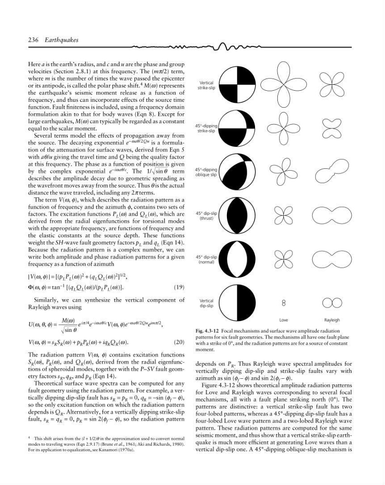
Fig. 4.3-12 Focal mechanisms and surface wave amplitude radiation
patterns for six fault geometries. The mechanisms all have one fault plane
with a strike of 0°, and the radiation patterns are for a source of constant
moment.
Vertical
strike-slip
45°-dipping
strike-slip
45°-dipping
oblique slip
45° dip-slip
(thrust)
45° dip-slip
(normal)
Vertical
dip-slip
Love
Rayleigh
depends on P R . Thus Rayleigh wave spectral amplitudes for
vertically dipping dip-slip and strike-slip faults vary with
azimuth as sin (φ f − φ) and sin 2(φ f − φ).
Figure 4.3-12 shows theoretical amplitude radiation patterns
for Love and Rayleigh waves corresponding to several focal
mechanisms, all with a fault plane striking north (0°). The
patterns are distinctive: a vertical strike-slip fault has two
four-lobed patterns, whereas a 45°-dipping dip-slip fault has a
four-lobed Love wave pattern and a two-lobed Rayleigh wave
pattern. These radiation patterns are computed for the same
seismic moment, and thus show that a vertical strike-slip earthquake is much more efficient at generating Love waves than a
vertical dip-slip one. A 45°-dipping oblique-slip mechanism is
4 This shift arises from the (l + 1/2)θ in the approximation used to convert normal
modes to traveling waves (Eqn 2.9.17) (Brune et al., 1961; Aki and Richards, 1980).
For its application to equalization, see Kanamori (1970a).
Here a is the earth’s radius, and c and u are the phase and group
velocities (Section 2.8.1) at this frequency. The (mπ/2) term,
where m is the number of times the wave passed the epicenter
or its antipode, is called the polar phase shift. 4 M(ω) represents
the earthquake’s seismic moment release as a function of
frequency, and thus can incorporate effects of the source time
function. Fault finiteness is included, using a frequency domain
formulation akin to that for body waves (Eqn 8). Except for
large earthquakes, M(ω) can typically be regarded as a constant
equal to the scalar moment.
Several terms model the effects of propagation away from
the source. The decaying exponential e −ωaθ/2Qu is a formulation of the attenuation for surface waves, derived from Eqn 5
with aθ/u giving the travel time and Q being the quality factor
at this frequency. The phase as a function of position is given
by the complex exponential e −iωaθ/c . The 1/ sin θ term
describes the amplitude decay due to geometric spreading as
the wavefront moves away from the source. Thus θ is the actual
distance the wave traveled, including any 2π terms.
The term V(ω, φ), which describes the radiation pattern as a
function of frequency and the azimuth φ, contains two sets of
factors. The excitation functions P L (ω) and Q L (ω), which are
derived from the radial eigenfunctions for torsional modes
with the appropriate frequency, are functions of frequency and
the elastic constants at the source depth. These functions
weight the SH-wave fault geometry factors p L and q L (Eqn 14).
Because the radiation pattern is a complex number, we can
write both amplitude and phase radiation patterns for a given
frequency as a function of azimuth
|V(ω, φ) | = [(p L P L (ω)) 2 + (q L Q L (ω)) 2 ] 1/2 ,
Φ(ω, φ) = tan −1 [(q L Q L (ω))/(p L P L (ω))].
(19)
Similarly, we can synthesize the vertical component of
Rayleigh waves using
U(ω, θ, φ) =
M( )
sin
ω
θ
e iπ /4 e −iω aθ /c V(ω, φ)e −ω aθ /2Qu e imπ/2 ,
V(ω, φ) = s R S R (ω) + p R P R (ω) + iq R Q R (ω).
(20)
The radiation pattern V(ω, φ) contains excitation functions
S R (ω), P R (ω), and Q R (ω), derived from the radial eigenfunctions of spheroidal modes, together with the P–SV fault geometry factors s R , q R , and p R (Eqn 14).
Theoretical surface wave spectra can be computed for any
fault geometry using the radiation pattern. For example, a vertically dipping dip-slip fault has s R = p R = 0, q R = −sin (φ f − φ),
so the only excitation function on which the radiation pattern
depends is Q R . Alternatively, for a vertically dipping strike-slip
fault, s R = q R = 0, p R = sin 2(φ f − φ), so the radiation pattern
Fig. 4.3-12 Focal mechanisms and surface wave amplitude radiation
patterns for six fault geometries. The mechanisms all have one fault plane
with a strike of 0°, and the radiation patterns are for a source of constant
moment.
Vertical
strike-slip
45°-dipping
strike-slip
45°-dipping
oblique slip
45° dip-slip
(thrust)
45° dip-slip
(normal)
Vertical
dip-slip
Love
Rayleigh
depends on P R . Thus Rayleigh wave spectral amplitudes for
vertically dipping dip-slip and strike-slip faults vary with
azimuth as sin (φ f − φ) and sin 2(φ f − φ).
Figure 4.3-12 shows theoretical amplitude radiation patterns
for Love and Rayleigh waves corresponding to several focal
mechanisms, all with a fault plane striking north (0°). The
patterns are distinctive: a vertical strike-slip fault has two
four-lobed patterns, whereas a 45°-dipping dip-slip fault has a
four-lobed Love wave pattern and a two-lobed Rayleigh wave
pattern. These radiation patterns are computed for the same
seismic moment, and thus show that a vertical strike-slip earthquake is much more efficient at generating Love waves than a
vertical dip-slip one. A 45°-dipping oblique-slip mechanism is
4 This shift arises from the (l + 1/2)θ in the approximation used to convert normal
modes to traveling waves (Eqn 2.9.17) (Brune et al., 1961; Aki and Richards, 1980).
For its application to equalization, see Kanamori (1970a).