

16°
15°
14°
88°
91°
90°
89°
0
50
100 km
0
Source time function
1
3
6
15 30 45 60 75 90 105 120
1
2
3
6
9
5
4
8
7
Data
Synthetic
120 s
Total
Caribbean
Sea
Mexico
Pacific
Ocean
M ot ag u a fa u lt
4.3 Waveform modeling 235
Fig. 4.3-10 Comparison of seismograms synthesized at a teleseismic
distance with different source time functions. The effects of the
seismometer and attenuation make it difficult to resolve some of the details
of the time function. (Stein and Kroeger, 1980. Reproduced with the
permission of the American Society of Mechanical Engineers.)
Synthetic
Source time function
5 s
30 s
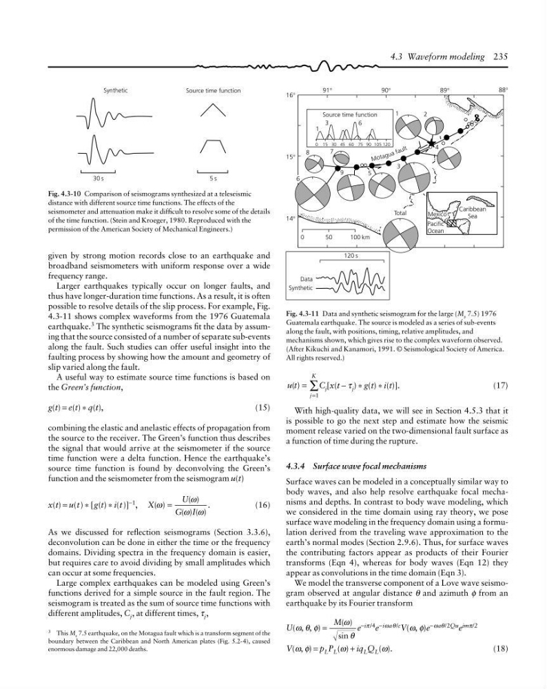
Fig. 4.3-11 Data and synthetic seismogram for the large (M s 7.5) 1976
Guatemala earthquake. The source is modeled as a series of sub-events
along the fault, with positions, timing, relative amplitudes, and
mechanisms shown, which gives rise to the complex waveform observed.
(After Kikuchi and Kanamori, 1991. © Seismological Society of America.
All rights reserved.)
given by strong motion records close to an earthquake and
broadband seismometers with uniform response over a wide
frequency range.
Larger earthquakes typically occur on longer faults, and
thus have longer-duration time functions. As a result, it is often
possible to resolve details of the slip process. For example, Fig.
4.3-11 shows complex waveforms from the 1976 Guatemala
earthquake. 3 The synthetic seismograms fit the data by assuming that the source consisted of a number of separate sub-events
along the fault. Such studies can offer useful insight into the
faulting process by showing how the amount and geometry of
slip varied along the fault.
A useful way to estimate source time functions is based on
the Green’s function,
g(t) = e(t) * q(t),
(15)
combining the elastic and anelastic effects of propagation from
the source to the receiver. The Green’s function thus describes
the signal that would arrive at the seismometer if the source
time function were a delta function. Hence the earthquake’s
source time function is found by deconvolving the Green’s
function and the seismometer from the seismogram u(t)
x(t) = u(t) * [g(t) * i(t )] −1 , X
U
G I
( )
( )
( ) ( )
.
ω
ω
ω ω
=
(16)
As we discussed for reflection seismograms (Section 3.3.6),
deconvolution can be done in either the time or the frequency
domains. Dividing spectra in the frequency domain is easier,
but requires care to avoid dividing by small amplitudes which
can occur at some frequencies.
Large complex earthquakes can be modeled using Green’s
functions derived for a simple source in the fault region. The
seismogram is treated as the sum of source time functions with
different amplitudes, C j , at different times, τ j ,
3 This M s 7.5 earthquake, on the Motagua fault which is a transform segment of the
boundary between the Caribbean and North American plates (Fig. 5.2-4), caused
enormous damage and 22,000 deaths.
u t
j
K
( ) =
=
∑
1
C j [x(t − τ j ) * g(t) * i(t)].
(17)
With high-quality data, we will see in Section 4.5.3 that it
is possible to go the next step and estimate how the seismic
moment release varied on the two-dimensional fault surface as
a function of time during the rupture.
4.3.4 Surface wave focal mechanisms
Surface waves can be modeled in a conceptually similar way to
body waves, and also help resolve earthquake focal mechanisms and depths. In contrast to body wave modeling, which
we considered in the time domain using ray theory, we pose
surface wave modeling in the frequency domain using a formulation derived from the traveling wave approximation to the
earth’s normal modes (Section 2.9.6). Thus, for surface waves
the contributing factors appear as products of their Fourier
transforms (Eqn 4), whereas for body waves (Eqn 12) they
appear as convolutions in the time domain (Eqn 3).
We model the transverse component of a Love wave seismogram observed at angular distance θ and azimuth φ from an
earthquake by its Fourier transform
U(ω, θ, φ) =
M( )
sin
ω
θ
e −iπ /4 e −iωaθ /c V(ω, φ)e −ωaθ/2Qu e imπ/2
V(ω, φ) = p L P L (ω) + iq L Q L (ω).
(18)
15°
14°
88°
91°
90°
89°
0
50
100 km
0
Source time function
1
3
6
15 30 45 60 75 90 105 120
1
2
3
6
9
5
4
8
7
Data
Synthetic
120 s
Total
Caribbean
Sea
Mexico
Pacific
Ocean
M ot ag u a fa u lt
4.3 Waveform modeling 235
Fig. 4.3-10 Comparison of seismograms synthesized at a teleseismic
distance with different source time functions. The effects of the
seismometer and attenuation make it difficult to resolve some of the details
of the time function. (Stein and Kroeger, 1980. Reproduced with the
permission of the American Society of Mechanical Engineers.)
Synthetic
Source time function
5 s
30 s
Fig. 4.3-11 Data and synthetic seismogram for the large (M s 7.5) 1976
Guatemala earthquake. The source is modeled as a series of sub-events
along the fault, with positions, timing, relative amplitudes, and
mechanisms shown, which gives rise to the complex waveform observed.
(After Kikuchi and Kanamori, 1991. © Seismological Society of America.
All rights reserved.)
given by strong motion records close to an earthquake and
broadband seismometers with uniform response over a wide
frequency range.
Larger earthquakes typically occur on longer faults, and
thus have longer-duration time functions. As a result, it is often
possible to resolve details of the slip process. For example, Fig.
4.3-11 shows complex waveforms from the 1976 Guatemala
earthquake. 3 The synthetic seismograms fit the data by assuming that the source consisted of a number of separate sub-events
along the fault. Such studies can offer useful insight into the
faulting process by showing how the amount and geometry of
slip varied along the fault.
A useful way to estimate source time functions is based on
the Green’s function,
g(t) = e(t) * q(t),
(15)
combining the elastic and anelastic effects of propagation from
the source to the receiver. The Green’s function thus describes
the signal that would arrive at the seismometer if the source
time function were a delta function. Hence the earthquake’s
source time function is found by deconvolving the Green’s
function and the seismometer from the seismogram u(t)
x(t) = u(t) * [g(t) * i(t )] −1 , X
U
G I
( )
( )
( ) ( )
.
ω
ω
ω ω
=
(16)
As we discussed for reflection seismograms (Section 3.3.6),
deconvolution can be done in either the time or the frequency
domains. Dividing spectra in the frequency domain is easier,
but requires care to avoid dividing by small amplitudes which
can occur at some frequencies.
Large complex earthquakes can be modeled using Green’s
functions derived for a simple source in the fault region. The
seismogram is treated as the sum of source time functions with
different amplitudes, C j , at different times, τ j ,
3 This M s 7.5 earthquake, on the Motagua fault which is a transform segment of the
boundary between the Caribbean and North American plates (Fig. 5.2-4), caused
enormous damage and 22,000 deaths.
u t
j
K
( ) =
=
∑
1
C j [x(t − τ j ) * g(t) * i(t)].
(17)
With high-quality data, we will see in Section 4.5.3 that it
is possible to go the next step and estimate how the seismic
moment release varied on the two-dimensional fault surface as
a function of time during the rupture.
4.3.4 Surface wave focal mechanisms
Surface waves can be modeled in a conceptually similar way to
body waves, and also help resolve earthquake focal mechanisms and depths. In contrast to body wave modeling, which
we considered in the time domain using ray theory, we pose
surface wave modeling in the frequency domain using a formulation derived from the traveling wave approximation to the
earth’s normal modes (Section 2.9.6). Thus, for surface waves
the contributing factors appear as products of their Fourier
transforms (Eqn 4), whereas for body waves (Eqn 12) they
appear as convolutions in the time domain (Eqn 3).
We model the transverse component of a Love wave seismogram observed at angular distance θ and azimuth φ from an
earthquake by its Fourier transform
U(ω, θ, φ) =
M( )
sin
ω
θ
e −iπ /4 e −iωaθ /c V(ω, φ)e −ωaθ/2Qu e imπ/2
V(ω, φ) = p L P L (ω) + iq L Q L (ω).
(18)