

234 Earthquakes
Without attenuation
and instrument response
20 40 60 80
Time (s)
Synthetic
seismogram
20 40 60 80
Time (s)
Data
10
20
30
40
50
Model depth (km)
Ocean
Halfspace
P w P
S w P
sP
pP
Direct P
Source
P
sP
P w P
pP
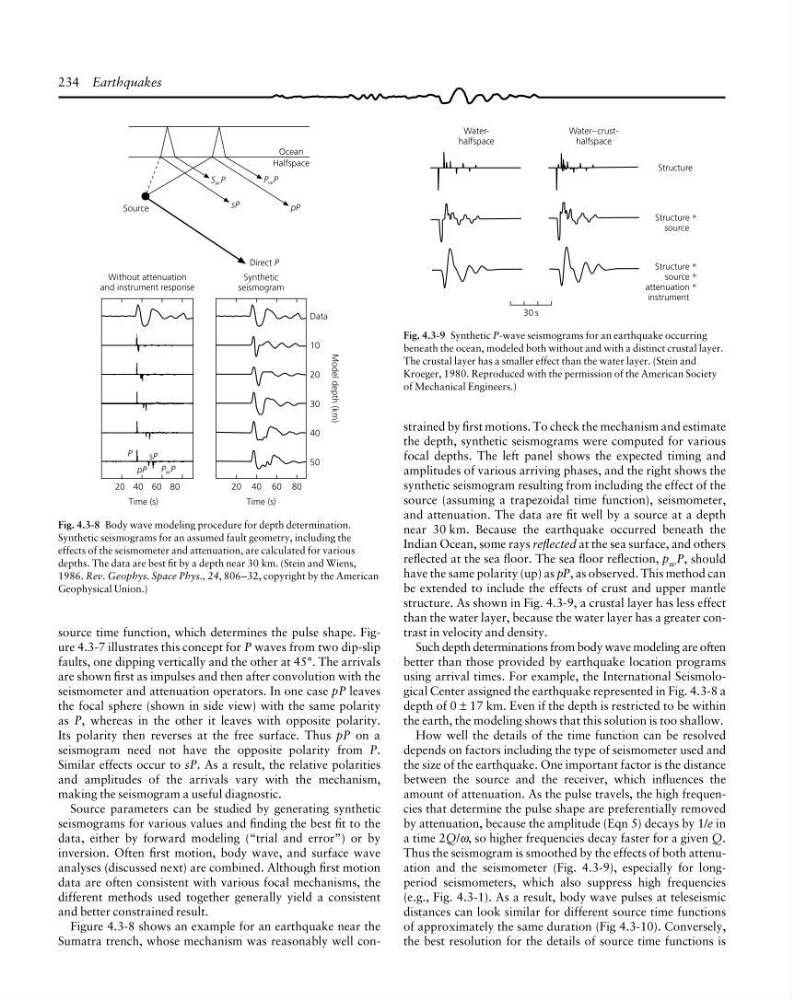
Fig. 4.3-8 Body wave modeling procedure for depth determination.
Synthetic seismograms for an assumed fault geometry, including the
effects of the seismometer and attenuation, are calculated for various
depths. The data are best fit by a depth near 30 km. (Stein and Wiens,
1986. Rev. Geophys. Space Phys., 24, 806–32, copyright by the American
Geophysical Union.)
source time function, which determines the pulse shape. Figure 4.3-7 illustrates this concept for P waves from two dip-slip
faults, one dipping vertically and the other at 45°. The arrivals
are shown first as impulses and then after convolution with the
seismometer and attenuation operators. In one case pP leaves
the focal sphere (shown in side view) with the same polarity
as P, whereas in the other it leaves with opposite polarity.
Its polarity then reverses at the free surface. Thus pP on a
seismogram need not have the opposite polarity from P.
Similar effects occur to sP. As a result, the relative polarities
and amplitudes of the arrivals vary with the mechanism,
making the seismogram a useful diagnostic.
Source parameters can be studied by generating synthetic
seismograms for various values and finding the best fit to the
data, either by forward modeling (“trial and error”) or by
inversion. Often first motion, body wave, and surface wave
analyses (discussed next) are combined. Although first motion
data are often consistent with various focal mechanisms, the
different methods used together generally yield a consistent
and better constrained result.
Figure 4.3-8 shows an example for an earthquake near the
Sumatra trench, whose mechanism was reasonably well con30 s
Structure
Structure *
source
Structure *
source *
attenuation *
instrument
Waterhalfspace
Water–crusthalfspace
Fig. 4.3-9 Synthetic P-wave seismograms for an earthquake occurring
beneath the ocean, modeled both without and with a distinct crustal layer.
The crustal layer has a smaller effect than the water layer. (Stein and
Kroeger, 1980. Reproduced with the permission of the American Society
of Mechanical Engineers.)
strained by first motions. To check the mechanism and estimate
the depth, synthetic seismograms were computed for various
focal depths. The left panel shows the expected timing and
amplitudes of various arriving phases, and the right shows the
synthetic seismogram resulting from including the effect of the
source (assuming a trapezoidal time function), seismometer,
and attenuation. The data are fit well by a source at a depth
near 30 km. Because the earthquake occurred beneath the
Indian Ocean, some rays reflected at the sea surface, and others
reflected at the sea floor. The sea floor reflection, p w P, should
have the same polarity (up) as pP, as observed. This method can
be extended to include the effects of crust and upper mantle
structure. As shown in Fig. 4.3-9, a crustal layer has less effect
than the water layer, because the water layer has a greater contrast in velocity and density.
Such depth determinations from body wave modeling are often
better than those provided by earthquake location programs
using arrival times. For example, the International Seismological Center assigned the earthquake represented in Fig. 4.3-8 a
depth of 0 ± 17 km. Even if the depth is restricted to be within
the earth, the modeling shows that this solution is too shallow.
How well the details of the time function can be resolved
depends on factors including the type of seismometer used and
the size of the earthquake. One important factor is the distance
between the source and the receiver, which influences the
amount of attenuation. As the pulse travels, the high frequencies that determine the pulse shape are preferentially removed
by attenuation, because the amplitude (Eqn 5) decays by 1/e in
a time 2Q/ω, so higher frequencies decay faster for a given Q.
Thus the seismogram is smoothed by the effects of both attenuation and the seismometer (Fig. 4.3-9), especially for longperiod seismometers, which also suppress high frequencies
(e.g., Fig. 4.3-1). As a result, body wave pulses at teleseismic
distances can look similar for different source time functions
of approximately the same duration (Fig 4.3-10). Conversely,
the best resolution for the details of source time functions is
Without attenuation
and instrument response
20 40 60 80
Time (s)
Synthetic
seismogram
20 40 60 80
Time (s)
Data
10
20
30
40
50
Model depth (km)
Ocean
Halfspace
P w P
S w P
sP
pP
Direct P
Source
P
sP
P w P
pP
Fig. 4.3-8 Body wave modeling procedure for depth determination.
Synthetic seismograms for an assumed fault geometry, including the
effects of the seismometer and attenuation, are calculated for various
depths. The data are best fit by a depth near 30 km. (Stein and Wiens,
1986. Rev. Geophys. Space Phys., 24, 806–32, copyright by the American
Geophysical Union.)
source time function, which determines the pulse shape. Figure 4.3-7 illustrates this concept for P waves from two dip-slip
faults, one dipping vertically and the other at 45°. The arrivals
are shown first as impulses and then after convolution with the
seismometer and attenuation operators. In one case pP leaves
the focal sphere (shown in side view) with the same polarity
as P, whereas in the other it leaves with opposite polarity.
Its polarity then reverses at the free surface. Thus pP on a
seismogram need not have the opposite polarity from P.
Similar effects occur to sP. As a result, the relative polarities
and amplitudes of the arrivals vary with the mechanism,
making the seismogram a useful diagnostic.
Source parameters can be studied by generating synthetic
seismograms for various values and finding the best fit to the
data, either by forward modeling (“trial and error”) or by
inversion. Often first motion, body wave, and surface wave
analyses (discussed next) are combined. Although first motion
data are often consistent with various focal mechanisms, the
different methods used together generally yield a consistent
and better constrained result.
Figure 4.3-8 shows an example for an earthquake near the
Sumatra trench, whose mechanism was reasonably well con30 s
Structure
Structure *
source
Structure *
source *
attenuation *
instrument
Waterhalfspace
Water–crusthalfspace
Fig. 4.3-9 Synthetic P-wave seismograms for an earthquake occurring
beneath the ocean, modeled both without and with a distinct crustal layer.
The crustal layer has a smaller effect than the water layer. (Stein and
Kroeger, 1980. Reproduced with the permission of the American Society
of Mechanical Engineers.)
strained by first motions. To check the mechanism and estimate
the depth, synthetic seismograms were computed for various
focal depths. The left panel shows the expected timing and
amplitudes of various arriving phases, and the right shows the
synthetic seismogram resulting from including the effect of the
source (assuming a trapezoidal time function), seismometer,
and attenuation. The data are fit well by a source at a depth
near 30 km. Because the earthquake occurred beneath the
Indian Ocean, some rays reflected at the sea surface, and others
reflected at the sea floor. The sea floor reflection, p w P, should
have the same polarity (up) as pP, as observed. This method can
be extended to include the effects of crust and upper mantle
structure. As shown in Fig. 4.3-9, a crustal layer has less effect
than the water layer, because the water layer has a greater contrast in velocity and density.
Such depth determinations from body wave modeling are often
better than those provided by earthquake location programs
using arrival times. For example, the International Seismological Center assigned the earthquake represented in Fig. 4.3-8 a
depth of 0 ± 17 km. Even if the depth is restricted to be within
the earth, the modeling shows that this solution is too shallow.
How well the details of the time function can be resolved
depends on factors including the type of seismometer used and
the size of the earthquake. One important factor is the distance
between the source and the receiver, which influences the
amount of attenuation. As the pulse travels, the high frequencies that determine the pulse shape are preferentially removed
by attenuation, because the amplitude (Eqn 5) decays by 1/e in
a time 2Q/ω, so higher frequencies decay faster for a given Q.
Thus the seismogram is smoothed by the effects of both attenuation and the seismometer (Fig. 4.3-9), especially for longperiod seismometers, which also suppress high frequencies
(e.g., Fig. 4.3-1). As a result, body wave pulses at teleseismic
distances can look similar for different source time functions
of approximately the same duration (Fig 4.3-10). Conversely,
the best resolution for the details of source time functions is