

232 Earthquakes
Source
x(t)
Structure
q(t)
Instrument
i(t)
Seismogram
u(t)
*
*
=
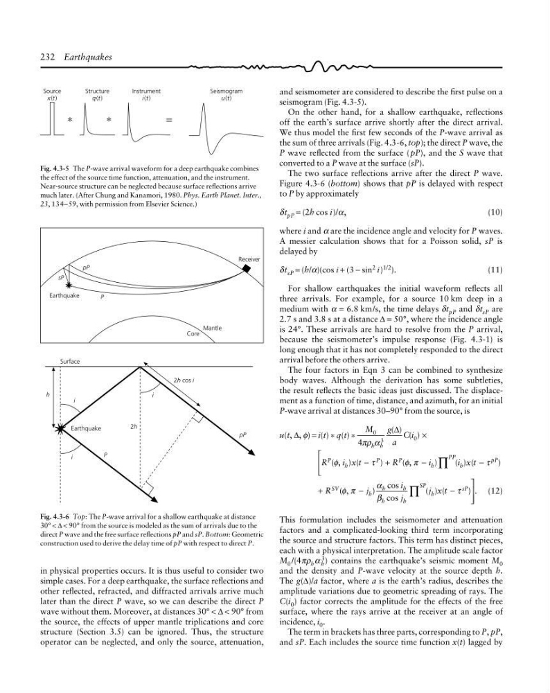
and seismometer are considered to describe the first pulse on a
seismogram (Fig. 4.3-5).
On the other hand, for a shallow earthquake, reflections
off the earth’s surface arrive shortly after the direct arrival.
We thus model the first few seconds of the P-wave arrival as
the sum of three arrivals (Fig. 4.3-6, top); the direct P wave, the
P wave reflected from the surface ( pP), and the S wave that
converted to a P wave at the surface (sP).
The two surface reflections arrive after the direct P wave.
Figure 4.3-6 (bottom) shows that pP is delayed with respect
to P by approximately
δt pP = (2h cos i)/α,
(10)
where i and α are the incidence angle and velocity for P waves.
A messier calculation shows that for a Poisson solid, sP is
delayed by
δt sP = (h/α)(cos i + (3 − sin
2 i)
1/2
).
(11)
For shallow earthquakes the initial waveform reflects all
three arrivals. For example, for a source 10 km deep in a
medium with α = 6.8 km/s, the time delays δt pP and δt sP are
2.7 s and 3.8 s at a distance ∆ = 50°, where the incidence angle
is 24°. These arrivals are hard to resolve from the P arrival,
because the seismometer’s impulse response (Fig. 4.3-1) is
long enough that it has not completely responded to the direct
arrival before the others arrive.
The four factors in Eqn 3 can be combined to synthesize
body waves. Although the derivation has some subtleties,
the result reflects the basic ideas just discussed. The displacement as a function of time, distance, and azimuth, for an initial
P-wave arrival at distances 30–90° from the source, is
u(t, ∆, φ) = i(t) * q(t) *
M
g
a
C i
h h
0
3
0
4πρ α
( ) ( )
∆
×
−
+
−
−
⎡
⎣
⎢
⎢
∏
( , ) (
)
( ,
)
( ) (
)
R
i xt
R
i
i xt
P
h
P
P
h
PP
h
pP
φ
τ
φ π
τ
+
−
−
⎤
⎦
⎥
⎥
∏
( ,
)
cos
cos
( ) (
) .
R
j
i
j
j x t
SV
h
h
h
h
h
SP
h
sP
φ π
α
β
τ
(12)
This formulation includes the seismometer and attenuation
factors and a complicated-looking third term incorporating
the source and structure factors. This term has distinct pieces,
each with a physical interpretation. The amplitude scale factor
M 0 /(4πρ h α
3
h ) contains the earthquake’s seismic moment M 0
and the density and P-wave velocity at the source depth h.
The g(∆)/a factor, where a is the earth’s radius, describes the
amplitude variations due to geometric spreading of rays. The
C(i 0 ) factor corrects the amplitude for the effects of the free
surface, where the rays arrive at the receiver at an angle of
incidence, i 0 .
The term in brackets has three parts, corresponding to P, pP,
and sP. Each includes the source time function x(t) lagged by
Fig. 4.3-6 Top: The P-wave arrival for a shallow earthquake at distance
30° < ∆ < 90° from the source is modeled as the sum of arrivals due to the
direct P wave and the free surface reflections pP and sP. Bottom: Geometric
construction used to derive the delay time of pP with respect to direct P.
Receiver
Earthquake
pP
sP
P
Mantle
Core
Surface
h
i
i
P
i
pP
2h cos i
2h
Earthquake
Fig. 4.3-5 The P-wave arrival waveform for a deep earthquake combines
the effect of the source time function, attenuation, and the instrument.
Near-source structure can be neglected because surface reflections arrive
much later. (After Chung and Kanamori, 1980. Phys. Earth Planet. Inter.,
23, 134–59, with permission from Elsevier Science.)
in physical properties occurs. It is thus useful to consider two
simple cases. For a deep earthquake, the surface reflections and
other reflected, refracted, and diffracted arrivals arrive much
later than the direct P wave, so we can describe the direct P
wave without them. Moreover, at distances 30° < ∆ < 90° from
the source, the effects of upper mantle triplications and core
structure (Section 3.5) can be ignored. Thus, the structure
operator can be neglected, and only the source, attenuation,
Source
x(t)
Structure
q(t)
Instrument
i(t)
Seismogram
u(t)
*
*
=
and seismometer are considered to describe the first pulse on a
seismogram (Fig. 4.3-5).
On the other hand, for a shallow earthquake, reflections
off the earth’s surface arrive shortly after the direct arrival.
We thus model the first few seconds of the P-wave arrival as
the sum of three arrivals (Fig. 4.3-6, top); the direct P wave, the
P wave reflected from the surface ( pP), and the S wave that
converted to a P wave at the surface (sP).
The two surface reflections arrive after the direct P wave.
Figure 4.3-6 (bottom) shows that pP is delayed with respect
to P by approximately
δt pP = (2h cos i)/α,
(10)
where i and α are the incidence angle and velocity for P waves.
A messier calculation shows that for a Poisson solid, sP is
delayed by
δt sP = (h/α)(cos i + (3 − sin
2 i)
1/2
).
(11)
For shallow earthquakes the initial waveform reflects all
three arrivals. For example, for a source 10 km deep in a
medium with α = 6.8 km/s, the time delays δt pP and δt sP are
2.7 s and 3.8 s at a distance ∆ = 50°, where the incidence angle
is 24°. These arrivals are hard to resolve from the P arrival,
because the seismometer’s impulse response (Fig. 4.3-1) is
long enough that it has not completely responded to the direct
arrival before the others arrive.
The four factors in Eqn 3 can be combined to synthesize
body waves. Although the derivation has some subtleties,
the result reflects the basic ideas just discussed. The displacement as a function of time, distance, and azimuth, for an initial
P-wave arrival at distances 30–90° from the source, is
u(t, ∆, φ) = i(t) * q(t) *
M
g
a
C i
h h
0
3
0
4πρ α
( ) ( )
∆
×
−
+
−
−
⎡
⎣
⎢
⎢
∏
( , ) (
)
( ,
)
( ) (
)
R
i xt
R
i
i xt
P
h
P
P
h
PP
h
pP
φ
τ
φ π
τ
+
−
−
⎤
⎦
⎥
⎥
∏
( ,
)
cos
cos
( ) (
) .
R
j
i
j
j x t
SV
h
h
h
h
h
SP
h
sP
φ π
α
β
τ
(12)
This formulation includes the seismometer and attenuation
factors and a complicated-looking third term incorporating
the source and structure factors. This term has distinct pieces,
each with a physical interpretation. The amplitude scale factor
M 0 /(4πρ h α
3
h ) contains the earthquake’s seismic moment M 0
and the density and P-wave velocity at the source depth h.
The g(∆)/a factor, where a is the earth’s radius, describes the
amplitude variations due to geometric spreading of rays. The
C(i 0 ) factor corrects the amplitude for the effects of the free
surface, where the rays arrive at the receiver at an angle of
incidence, i 0 .
The term in brackets has three parts, corresponding to P, pP,
and sP. Each includes the source time function x(t) lagged by
Fig. 4.3-6 Top: The P-wave arrival for a shallow earthquake at distance
30° < ∆ < 90° from the source is modeled as the sum of arrivals due to the
direct P wave and the free surface reflections pP and sP. Bottom: Geometric
construction used to derive the delay time of pP with respect to direct P.
Receiver
Earthquake
pP
sP
P
Mantle
Core
Surface
h
i
i
P
i
pP
2h cos i
2h
Earthquake
Fig. 4.3-5 The P-wave arrival waveform for a deep earthquake combines
the effect of the source time function, attenuation, and the instrument.
Near-source structure can be neglected because surface reflections arrive
much later. (After Chung and Kanamori, 1980. Phys. Earth Planet. Inter.,
23, 134–59, with permission from Elsevier Science.)
in physical properties occurs. It is thus useful to consider two
simple cases. For a deep earthquake, the surface reflections and
other reflected, refracted, and diffracted arrivals arrive much
later than the direct P wave, so we can describe the direct P
wave without them. Moreover, at distances 30° < ∆ < 90° from
the source, the effects of upper mantle triplications and core
structure (Section 3.5) can be ignored. Thus, the structure
operator can be neglected, and only the source, attenuation,