

Area = M 0
= 180°
θ
Area = M 0
= 90°
θ
Area = M 0
= 270°
θ
Area
= M 0
= 0°
θ
Fault
Rupture
direction
4.3 Waveform modeling 231
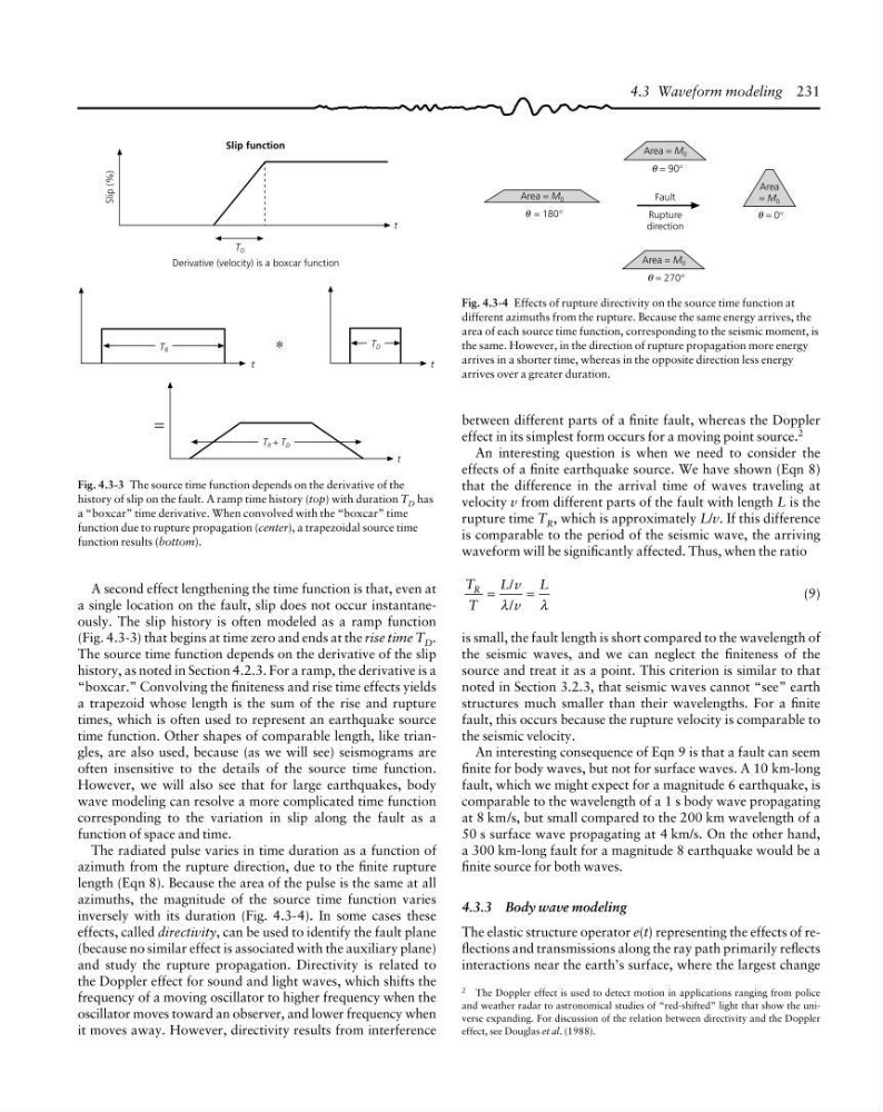
Fig. 4.3-4 Effects of rupture directivity on the source time function at
different azimuths from the rupture. Because the same energy arrives, the
area of each source time function, corresponding to the seismic moment, is
the same. However, in the direction of rupture propagation more energy
arrives in a shorter time, whereas in the opposite direction less energy
arrives over a greater duration.
A second effect lengthening the time function is that, even at
a single location on the fault, slip does not occur instantaneously. The slip history is often modeled as a ramp function
(Fig. 4.3-3) that begins at time zero and ends at the rise time T D .
The source time function depends on the derivative of the slip
history, as noted in Section 4.2.3. For a ramp, the derivative is a
“boxcar.” Convolving the finiteness and rise time effects yields
a trapezoid whose length is the sum of the rise and rupture
times, which is often used to represent an earthquake source
time function. Other shapes of comparable length, like triangles, are also used, because (as we will see) seismograms are
often insensitive to the details of the source time function.
However, we will also see that for large earthquakes, body
wave modeling can resolve a more complicated time function
corresponding to the variation in slip along the fault as a
function of space and time.
The radiated pulse varies in time duration as a function of
azimuth from the rupture direction, due to the finite rupture
length (Eqn 8). Because the area of the pulse is the same at all
azimuths, the magnitude of the source time function varies
inversely with its duration (Fig. 4.3-4). In some cases these
effects, called directivity, can be used to identify the fault plane
(because no similar effect is associated with the auxiliary plane)
and study the rupture propagation. Directivity is related to
the Doppler effect for sound and light waves, which shifts the
frequency of a moving oscillator to higher frequency when the
oscillator moves toward an observer, and lower frequency when
it moves away. However, directivity results from interference
between different parts of a finite fault, whereas the Doppler
effect in its simplest form occurs for a moving point source. 2
An interesting question is when we need to consider the
effects of a finite earthquake source. We have shown (Eqn 8)
that the difference in the arrival time of waves traveling at
velocity v from different parts of the fault with length L is the
rupture time T R , which is approximately L/v. If this difference
is comparable to the period of the seismic wave, the arriving
waveform will be significantly affected. Thus, when the ratio
T
T
L v
v
L
R
/
/
=
=
λ
λ
(9)
is small, the fault length is short compared to the wavelength of
the seismic waves, and we can neglect the finiteness of the
source and treat it as a point. This criterion is similar to that
noted in Section 3.2.3, that seismic waves cannot “see” earth
structures much smaller than their wavelengths. For a finite
fault, this occurs because the rupture velocity is comparable to
the seismic velocity.
An interesting consequence of Eqn 9 is that a fault can seem
finite for body waves, but not for surface waves. A 10 km-long
fault, which we might expect for a magnitude 6 earthquake, is
comparable to the wavelength of a 1 s body wave propagating
at 8 km/s, but small compared to the 200 km wavelength of a
50 s surface wave propagating at 4 km/s. On the other hand,
a 300 km-long fault for a magnitude 8 earthquake would be a
finite source for both waves.
4.3.3 Body wave modeling
The elastic structure operator e(t) representing the effects of reflections and transmissions along the ray path primarily reflects
interactions near the earth’s surface, where the largest change
2 The Doppler effect is used to detect motion in applications ranging from police
and weather radar to astronomical studies of “red-shifted” light that show the universe expanding. For discussion of the relation between directivity and the Doppler
effect, see Douglas et al. (1988).
Slip (%)
T D
t
Slip function
Derivative (velocity) is a boxcar function
T R
t
T D
t
T R + T D
t
=
*
Fig. 4.3-3 The source time function depends on the derivative of the
history of slip on the fault. A ramp time history (top) with duration T D has
a “boxcar” time derivative. When convolved with the “boxcar” time
function due to rupture propagation (center), a trapezoidal source time
function results (bottom).
= 180°
θ
Area = M 0
= 90°
θ
Area = M 0
= 270°
θ
Area
= M 0
= 0°
θ
Fault
Rupture
direction
4.3 Waveform modeling 231
Fig. 4.3-4 Effects of rupture directivity on the source time function at
different azimuths from the rupture. Because the same energy arrives, the
area of each source time function, corresponding to the seismic moment, is
the same. However, in the direction of rupture propagation more energy
arrives in a shorter time, whereas in the opposite direction less energy
arrives over a greater duration.
A second effect lengthening the time function is that, even at
a single location on the fault, slip does not occur instantaneously. The slip history is often modeled as a ramp function
(Fig. 4.3-3) that begins at time zero and ends at the rise time T D .
The source time function depends on the derivative of the slip
history, as noted in Section 4.2.3. For a ramp, the derivative is a
“boxcar.” Convolving the finiteness and rise time effects yields
a trapezoid whose length is the sum of the rise and rupture
times, which is often used to represent an earthquake source
time function. Other shapes of comparable length, like triangles, are also used, because (as we will see) seismograms are
often insensitive to the details of the source time function.
However, we will also see that for large earthquakes, body
wave modeling can resolve a more complicated time function
corresponding to the variation in slip along the fault as a
function of space and time.
The radiated pulse varies in time duration as a function of
azimuth from the rupture direction, due to the finite rupture
length (Eqn 8). Because the area of the pulse is the same at all
azimuths, the magnitude of the source time function varies
inversely with its duration (Fig. 4.3-4). In some cases these
effects, called directivity, can be used to identify the fault plane
(because no similar effect is associated with the auxiliary plane)
and study the rupture propagation. Directivity is related to
the Doppler effect for sound and light waves, which shifts the
frequency of a moving oscillator to higher frequency when the
oscillator moves toward an observer, and lower frequency when
it moves away. However, directivity results from interference
between different parts of a finite fault, whereas the Doppler
effect in its simplest form occurs for a moving point source. 2
An interesting question is when we need to consider the
effects of a finite earthquake source. We have shown (Eqn 8)
that the difference in the arrival time of waves traveling at
velocity v from different parts of the fault with length L is the
rupture time T R , which is approximately L/v. If this difference
is comparable to the period of the seismic wave, the arriving
waveform will be significantly affected. Thus, when the ratio
T
T
L v
v
L
R
/
/
=
=
λ
λ
(9)
is small, the fault length is short compared to the wavelength of
the seismic waves, and we can neglect the finiteness of the
source and treat it as a point. This criterion is similar to that
noted in Section 3.2.3, that seismic waves cannot “see” earth
structures much smaller than their wavelengths. For a finite
fault, this occurs because the rupture velocity is comparable to
the seismic velocity.
An interesting consequence of Eqn 9 is that a fault can seem
finite for body waves, but not for surface waves. A 10 km-long
fault, which we might expect for a magnitude 6 earthquake, is
comparable to the wavelength of a 1 s body wave propagating
at 8 km/s, but small compared to the 200 km wavelength of a
50 s surface wave propagating at 4 km/s. On the other hand,
a 300 km-long fault for a magnitude 8 earthquake would be a
finite source for both waves.
4.3.3 Body wave modeling
The elastic structure operator e(t) representing the effects of reflections and transmissions along the ray path primarily reflects
interactions near the earth’s surface, where the largest change
2 The Doppler effect is used to detect motion in applications ranging from police
and weather radar to astronomical studies of “red-shifted” light that show the universe expanding. For discussion of the relation between directivity and the Doppler
effect, see Douglas et al. (1988).
Slip (%)
T D
t
Slip function
Derivative (velocity) is a boxcar function
T R
t
T D
t
T R + T D
t
=
*
Fig. 4.3-3 The source time function depends on the derivative of the
history of slip on the fault. A ramp time history (top) with duration T D has
a “boxcar” time derivative. When convolved with the “boxcar” time
function due to rupture propagation (center), a trapezoidal source time
function results (bottom).