

230 Earthquakes
Rupture
starts
Station
Rupture
direction
L
r 0
r
θ
v R
t
“Boxcar”
time pulse
T R = L(1/v R – cos /v )
θ
50
Gain
1500
1000
500
100
150
200
Period (s)
2
Amplitude
200
100
0
–100
4
6
8
Time (s)
Instrument response (WWSSN 15-100)
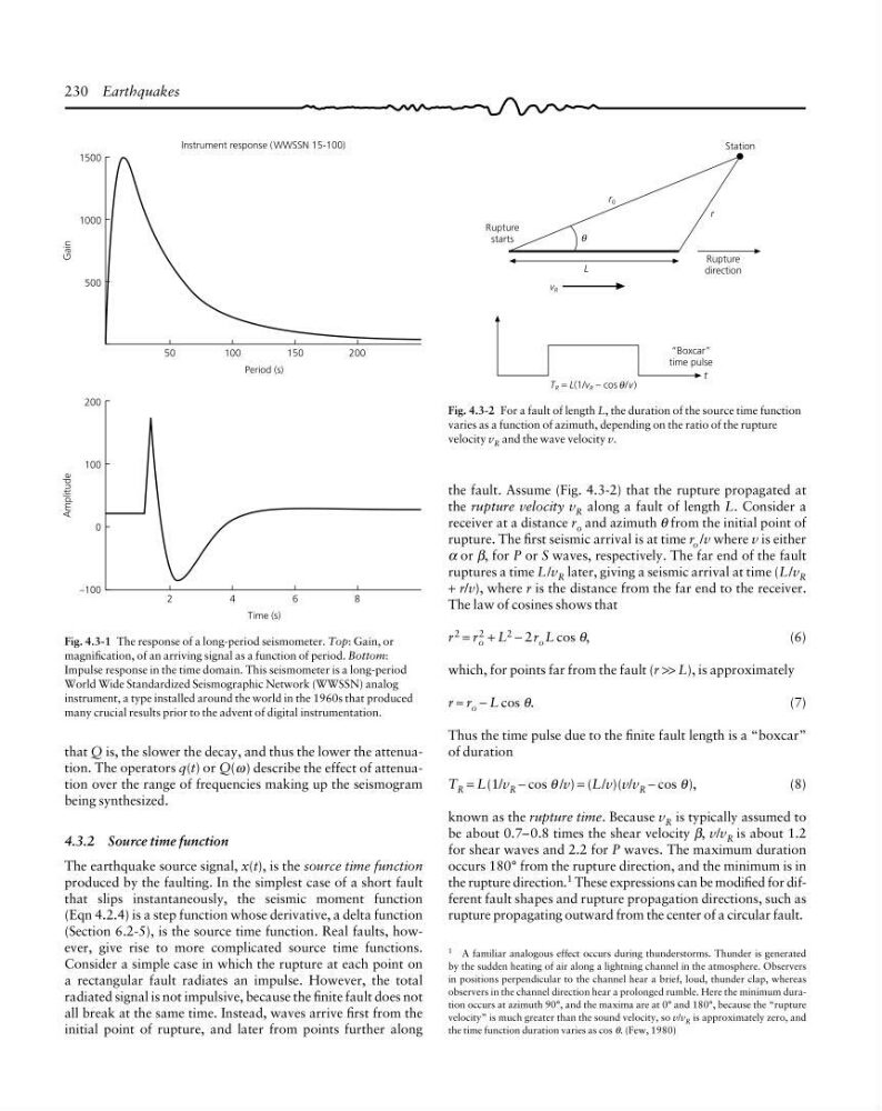
Fig. 4.3-1 The response of a long-period seismometer. Top: Gain, or
magnification, of an arriving signal as a function of period. Bottom:
Impulse response in the time domain. This seismometer is a long-period
World Wide Standardized Seismographic Network (WWSSN) analog
instrument, a type installed around the world in the 1960s that produced
many crucial results prior to the advent of digital instrumentation.
Fig. 4.3-2 For a fault of length L, the duration of the source time function
varies as a function of azimuth, depending on the ratio of the rupture
velocity v R and the wave velocity v.
1 A familiar analogous effect occurs during thunderstorms. Thunder is generated
by the sudden heating of air along a lightning channel in the atmosphere. Observers
in positions perpendicular to the channel hear a brief, loud, thunder clap, whereas
observers in the channel direction hear a prolonged rumble. Here the minimum duration occurs at azimuth 90°, and the maxima are at 0° and 180°, because the “rupture
velocity” is much greater than the sound velocity, so v/v R is approximately zero, and
the time function duration varies as cos θ. (Few, 1980)
that Q is, the slower the decay, and thus the lower the attenuation. The operators q(t) or Q(ω) describe the effect of attenuation over the range of frequencies making up the seismogram
being synthesized.
4.3.2 Source time function
The earthquake source signal, x(t), is the source time function
produced by the faulting. In the simplest case of a short fault
that slips instantaneously, the seismic moment function
(Eqn 4.2.4) is a step function whose derivative, a delta function
(Section 6.2-5), is the source time function. Real faults, however, give rise to more complicated source time functions.
Consider a simple case in which the rupture at each point on
a rectangular fault radiates an impulse. However, the total
radiated signal is not impulsive, because the finite fault does not
all break at the same time. Instead, waves arrive first from the
initial point of rupture, and later from points further along
the fault. Assume (Fig. 4.3-2) that the rupture propagated at
the rupture velocity v R along a fault of length L. Consider a
receiver at a distance r o and azimuth θ from the initial point of
rupture. The first seismic arrival is at time r o /v where v is either
α or β, for P or S waves, respectively. The far end of the fault
ruptures a time L/v R later, giving a seismic arrival at time (L/v R
+ r/v), where r is the distance from the far end to the receiver.
The law of cosines shows that
r
2
= r
2
o + L
2
− 2r o L cos θ,
(6)
which, for points far from the fault (r >> L), is approximately
r ≈ r o − L cos θ.
(7)
Thus the time pulse due to the finite fault length is a “boxcar”
of duration
T R = L(1/v R − cos θ /v) = (L/v)(v/v R − cos θ),
(8)
known as the rupture time. Because v R is typically assumed to
be about 0.7–0.8 times the shear velocity β, v/v R is about 1.2
for shear waves and 2.2 for P waves. The maximum duration
occurs 180° from the rupture direction, and the minimum is in
the rupture direction. 1 These expressions can be modified for different fault shapes and rupture propagation directions, such as
rupture propagating outward from the center of a circular fault.
Rupture
starts
Station
Rupture
direction
L
r 0
r
θ
v R
t
“Boxcar”
time pulse
T R = L(1/v R – cos /v )
θ
50
Gain
1500
1000
500
100
150
200
Period (s)
2
Amplitude
200
100
0
–100
4
6
8
Time (s)
Instrument response (WWSSN 15-100)
Fig. 4.3-1 The response of a long-period seismometer. Top: Gain, or
magnification, of an arriving signal as a function of period. Bottom:
Impulse response in the time domain. This seismometer is a long-period
World Wide Standardized Seismographic Network (WWSSN) analog
instrument, a type installed around the world in the 1960s that produced
many crucial results prior to the advent of digital instrumentation.
Fig. 4.3-2 For a fault of length L, the duration of the source time function
varies as a function of azimuth, depending on the ratio of the rupture
velocity v R and the wave velocity v.
1 A familiar analogous effect occurs during thunderstorms. Thunder is generated
by the sudden heating of air along a lightning channel in the atmosphere. Observers
in positions perpendicular to the channel hear a brief, loud, thunder clap, whereas
observers in the channel direction hear a prolonged rumble. Here the minimum duration occurs at azimuth 90°, and the maxima are at 0° and 180°, because the “rupture
velocity” is much greater than the sound velocity, so v/v R is approximately zero, and
the time function duration varies as cos θ. (Few, 1980)
that Q is, the slower the decay, and thus the lower the attenuation. The operators q(t) or Q(ω) describe the effect of attenuation over the range of frequencies making up the seismogram
being synthesized.
4.3.2 Source time function
The earthquake source signal, x(t), is the source time function
produced by the faulting. In the simplest case of a short fault
that slips instantaneously, the seismic moment function
(Eqn 4.2.4) is a step function whose derivative, a delta function
(Section 6.2-5), is the source time function. Real faults, however, give rise to more complicated source time functions.
Consider a simple case in which the rupture at each point on
a rectangular fault radiates an impulse. However, the total
radiated signal is not impulsive, because the finite fault does not
all break at the same time. Instead, waves arrive first from the
initial point of rupture, and later from points further along
the fault. Assume (Fig. 4.3-2) that the rupture propagated at
the rupture velocity v R along a fault of length L. Consider a
receiver at a distance r o and azimuth θ from the initial point of
rupture. The first seismic arrival is at time r o /v where v is either
α or β, for P or S waves, respectively. The far end of the fault
ruptures a time L/v R later, giving a seismic arrival at time (L/v R
+ r/v), where r is the distance from the far end to the receiver.
The law of cosines shows that
r
2
= r
2
o + L
2
− 2r o L cos θ,
(6)
which, for points far from the fault (r >> L), is approximately
r ≈ r o − L cos θ.
(7)
Thus the time pulse due to the finite fault length is a “boxcar”
of duration
T R = L(1/v R − cos θ /v) = (L/v)(v/v R − cos θ),
(8)
known as the rupture time. Because v R is typically assumed to
be about 0.7–0.8 times the shear velocity β, v/v R is about 1.2
for shear waves and 2.2 for P waves. The maximum duration
occurs 180° from the rupture direction, and the minimum is in
the rupture direction. 1 These expressions can be modified for different fault shapes and rupture propagation directions, such as
rupture propagating outward from the center of a circular fault.