

224 Earthquakes
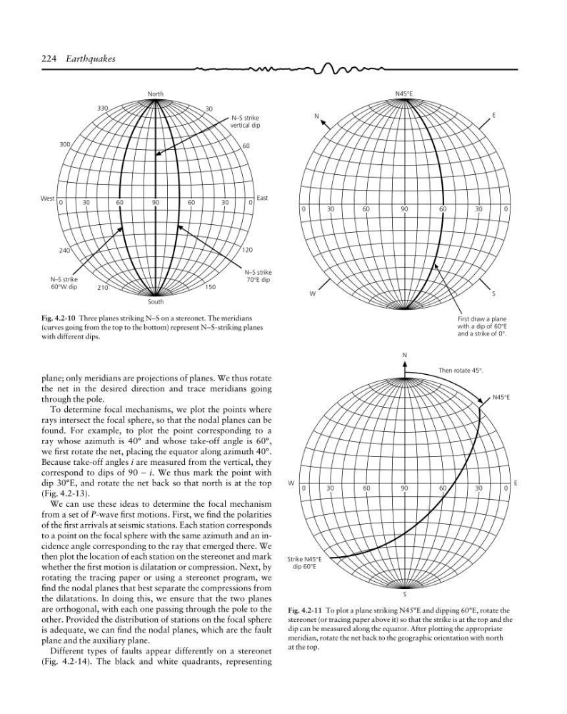
Fig. 4.2-10 Three planes striking N–S on a stereonet. The meridians
(curves going from the top to the bottom) represent N–S-striking planes
with different dips.
Fig. 4.2-11 To plot a plane striking N45°E and dipping 60°E, rotate the
stereonet (or tracing paper above it) so that the strike is at the top and the
dip can be measured along the equator. After plotting the appropriate
meridian, rotate the net back to the geographic orientation with north
at the top.
30
60
60
30
N45°E
First draw a plane
with a dip of 60°E
and a strike of 0°.
90
N
E
W
S
30
60
60
30
N45°E
90
W
E
N
S
Strike N45°E
dip 60°E
Then rotate 45°.
0
0
0
0
0
West
30
60
60
30
0
East
30
60
150
120
210
240
300
330
North
South
N–S strike
60°W dip
N–S strike
70°E dip
N–S strike
vertical dip
90
plane; only meridians are projections of planes. We thus rotate
the net in the desired direction and trace meridians going
through the pole.
To determine focal mechanisms, we plot the points where
rays intersect the focal sphere, so that the nodal planes can be
found. For example, to plot the point corresponding to a
ray whose azimuth is 40° and whose take-off angle is 60°,
we first rotate the net, placing the equator along azimuth 40°.
Because take-off angles i are measured from the vertical, they
correspond to dips of 90 − i. We thus mark the point with
dip 30°E, and rotate the net back so that north is at the top
(Fig. 4.2-13).
We can use these ideas to determine the focal mechanism
from a set of P-wave first motions. First, we find the polarities
of the first arrivals at seismic stations. Each station corresponds
to a point on the focal sphere with the same azimuth and an incidence angle corresponding to the ray that emerged there. We
then plot the location of each station on the stereonet and mark
whether the first motion is dilatation or compression. Next, by
rotating the tracing paper or using a stereonet program, we
find the nodal planes that best separate the compressions from
the dilatations. In doing this, we ensure that the two planes
are orthogonal, with each one passing through the pole to the
other. Provided the distribution of stations on the focal sphere
is adequate, we can find the nodal planes, which are the fault
plane and the auxiliary plane.
Different types of faults appear differently on a stereonet
(Fig. 4.2-14). The black and white quadrants, representing
Fig. 4.2-10 Three planes striking N–S on a stereonet. The meridians
(curves going from the top to the bottom) represent N–S-striking planes
with different dips.
Fig. 4.2-11 To plot a plane striking N45°E and dipping 60°E, rotate the
stereonet (or tracing paper above it) so that the strike is at the top and the
dip can be measured along the equator. After plotting the appropriate
meridian, rotate the net back to the geographic orientation with north
at the top.
30
60
60
30
N45°E
First draw a plane
with a dip of 60°E
and a strike of 0°.
90
N
E
W
S
30
60
60
30
N45°E
90
W
E
N
S
Strike N45°E
dip 60°E
Then rotate 45°.
0
0
0
0
0
West
30
60
60
30
0
East
30
60
150
120
210
240
300
330
North
South
N–S strike
60°W dip
N–S strike
70°E dip
N–S strike
vertical dip
90
plane; only meridians are projections of planes. We thus rotate
the net in the desired direction and trace meridians going
through the pole.
To determine focal mechanisms, we plot the points where
rays intersect the focal sphere, so that the nodal planes can be
found. For example, to plot the point corresponding to a
ray whose azimuth is 40° and whose take-off angle is 60°,
we first rotate the net, placing the equator along azimuth 40°.
Because take-off angles i are measured from the vertical, they
correspond to dips of 90 − i. We thus mark the point with
dip 30°E, and rotate the net back so that north is at the top
(Fig. 4.2-13).
We can use these ideas to determine the focal mechanism
from a set of P-wave first motions. First, we find the polarities
of the first arrivals at seismic stations. Each station corresponds
to a point on the focal sphere with the same azimuth and an incidence angle corresponding to the ray that emerged there. We
then plot the location of each station on the stereonet and mark
whether the first motion is dilatation or compression. Next, by
rotating the tracing paper or using a stereonet program, we
find the nodal planes that best separate the compressions from
the dilatations. In doing this, we ensure that the two planes
are orthogonal, with each one passing through the pole to the
other. Provided the distribution of stations on the focal sphere
is adequate, we can find the nodal planes, which are the fault
plane and the auxiliary plane.
Different types of faults appear differently on a stereonet
(Fig. 4.2-14). The black and white quadrants, representing