

3.8 Composition of the mantle and core 201
0.7
0.6
0.5
0.4
0.3
0.2
Uniform density
Density at a depth of 33 km
3.2
Shell
3.3
3.4
3.5
3.6
3.7
3.8
3.9
C
Ma
2 for the core
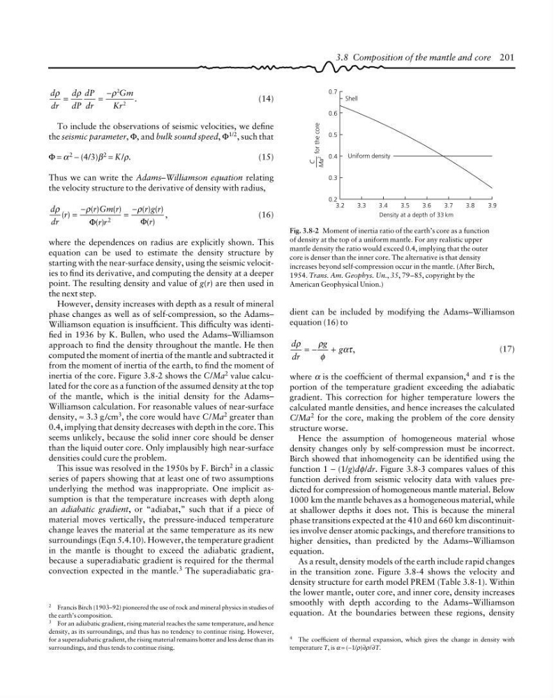
Fig. 3.8-2 Moment of inertia ratio of the earth’s core as a function
of density at the top of a uniform mantle. For any realistic upper
mantle density the ratio would exceed 0.4, implying that the outer
core is denser than the inner core. The alternative is that density
increases beyond self-compression occur in the mantle. (After Birch,
1954. Trans. Am. Geophys. Un., 35, 79–85, copyright by the
American Geophysical Union.)
d
dr
d
dP
dP
dr
Gm
Kr
ρ
ρ
ρ
.
=
=
−
2
2
(14)
To include the observations of seismic velocities, we define
the seismic parameter, Φ, and bulk sound speed, Φ 1/2 , such that
Φ = α 2 − (4/3)β 2 = K/ρ.
(15)
Thus we can write the Adams–Williamson equation relating
the velocity structure to the derivative of density with radius,
d
dr
r
r Gm r
r r
r g r
r
ρ
ρ
ρ
( )
( )
( )
( )
( ) ( )
( )
,
=
−
=
−
Φ
Φ
2
(16)
where the dependences on radius are explicitly shown. This
equation can be used to estimate the density structure by
starting with the near-surface density, using the seismic velocities to find its derivative, and computing the density at a deeper
point. The resulting density and value of g(r) are then used in
the next step.
However, density increases with depth as a result of mineral
phase changes as well as of self-compression, so the Adams–
Williamson equation is insufficient. This difficulty was identified in 1936 by K. Bullen, who used the Adams–Williamson
approach to find the density throughout the mantle. He then
computed the moment of inertia of the mantle and subtracted it
from the moment of inertia of the earth, to find the moment of
inertia of the core. Figure 3.8-2 shows the C/Ma 2 value calculated for the core as a function of the assumed density at the top
of the mantle, which is the initial density for the Adams–
Williamson calculation. For reasonable values of near-surface
density, ≈ 3.3 g /cm 3 , the core would have C/Ma 2 greater than
0.4, implying that density decreases with depth in the core. This
seems unlikely, because the solid inner core should be denser
than the liquid outer core. Only implausibly high near-surface
densities could cure the problem.
This issue was resolved in the 1950s by F. Birch
2 in a classic
series of papers showing that at least one of two assumptions
underlying the method was inappropriate. One implicit assumption is that the temperature increases with depth along
an adiabatic gradient, or “adiabat,” such that if a piece of
material moves vertically, the pressure-induced temperature
change leaves the material at the same temperature as its new
surroundings (Eqn 5.4.10). However, the temperature gradient
in the mantle is thought to exceed the adiabatic gradient,
because a superadiabatic gradient is required for the thermal
convection expected in the mantle. 3 The superadiabatic gra2 Francis Birch (1903–92) pioneered the use of rock and mineral physics in studies of
the earth’s composition.
3 For an adiabatic gradient, rising material reaches the same temperature, and hence
density, as its surroundings, and thus has no tendency to continue rising. However,
for a superadiabatic gradient, the rising material remains hotter and less dense than its
surroundings, and thus tends to continue rising.
4 The coefficient of thermal expansion, which gives the change in density with
temperature T, is α = (−1/ρ)∂ρ/∂T.
dient can be included by modifying the Adams–Williamson
equation (16) to
d
dr
g g
ρ
ρ
φ
ατ ,
= −
+
(17)
where α is the coefficient of thermal expansion,
4 and τ is the
portion of the temperature gradient exceeding the adiabatic
gradient. This correction for higher temperature lowers the
calculated mantle densities, and hence increases the calculated
C/Ma 2 for the core, making the problem of the core density
structure worse.
Hence the assumption of homogeneous material whose
density changes only by self-compression must be incorrect.
Birch showed that inhomogeneity can be identified using the
function 1 − (1/g)dφ/dr. Figure 3.8-3 compares values of this
function derived from seismic velocity data with values predicted for compression of homogeneous mantle material. Below
1000 km the mantle behaves as a homogeneous material, while
at shallower depths it does not. This is because the mineral
phase transitions expected at the 410 and 660 km discontinuities involve denser atomic packings, and therefore transitions to
higher densities, than predicted by the Adams–Williamson
equation.
As a result, density models of the earth include rapid changes
in the transition zone. Figure 3.8-4 shows the velocity and
density structure for earth model PREM (Table 3.8-1). Within
the lower mantle, outer core, and inner core, density increases
smoothly with depth according to the Adams–Williamson
equation. At the boundaries between these regions, density
0.7
0.6
0.5
0.4
0.3
0.2
Uniform density
Density at a depth of 33 km
3.2
Shell
3.3
3.4
3.5
3.6
3.7
3.8
3.9
C
Ma
2 for the core
Fig. 3.8-2 Moment of inertia ratio of the earth’s core as a function
of density at the top of a uniform mantle. For any realistic upper
mantle density the ratio would exceed 0.4, implying that the outer
core is denser than the inner core. The alternative is that density
increases beyond self-compression occur in the mantle. (After Birch,
1954. Trans. Am. Geophys. Un., 35, 79–85, copyright by the
American Geophysical Union.)
d
dr
d
dP
dP
dr
Gm
Kr
ρ
ρ
ρ
.
=
=
−
2
2
(14)
To include the observations of seismic velocities, we define
the seismic parameter, Φ, and bulk sound speed, Φ 1/2 , such that
Φ = α 2 − (4/3)β 2 = K/ρ.
(15)
Thus we can write the Adams–Williamson equation relating
the velocity structure to the derivative of density with radius,
d
dr
r
r Gm r
r r
r g r
r
ρ
ρ
ρ
( )
( )
( )
( )
( ) ( )
( )
,
=
−
=
−
Φ
Φ
2
(16)
where the dependences on radius are explicitly shown. This
equation can be used to estimate the density structure by
starting with the near-surface density, using the seismic velocities to find its derivative, and computing the density at a deeper
point. The resulting density and value of g(r) are then used in
the next step.
However, density increases with depth as a result of mineral
phase changes as well as of self-compression, so the Adams–
Williamson equation is insufficient. This difficulty was identified in 1936 by K. Bullen, who used the Adams–Williamson
approach to find the density throughout the mantle. He then
computed the moment of inertia of the mantle and subtracted it
from the moment of inertia of the earth, to find the moment of
inertia of the core. Figure 3.8-2 shows the C/Ma 2 value calculated for the core as a function of the assumed density at the top
of the mantle, which is the initial density for the Adams–
Williamson calculation. For reasonable values of near-surface
density, ≈ 3.3 g /cm 3 , the core would have C/Ma 2 greater than
0.4, implying that density decreases with depth in the core. This
seems unlikely, because the solid inner core should be denser
than the liquid outer core. Only implausibly high near-surface
densities could cure the problem.
This issue was resolved in the 1950s by F. Birch
2 in a classic
series of papers showing that at least one of two assumptions
underlying the method was inappropriate. One implicit assumption is that the temperature increases with depth along
an adiabatic gradient, or “adiabat,” such that if a piece of
material moves vertically, the pressure-induced temperature
change leaves the material at the same temperature as its new
surroundings (Eqn 5.4.10). However, the temperature gradient
in the mantle is thought to exceed the adiabatic gradient,
because a superadiabatic gradient is required for the thermal
convection expected in the mantle. 3 The superadiabatic gra2 Francis Birch (1903–92) pioneered the use of rock and mineral physics in studies of
the earth’s composition.
3 For an adiabatic gradient, rising material reaches the same temperature, and hence
density, as its surroundings, and thus has no tendency to continue rising. However,
for a superadiabatic gradient, the rising material remains hotter and less dense than its
surroundings, and thus tends to continue rising.
4 The coefficient of thermal expansion, which gives the change in density with
temperature T, is α = (−1/ρ)∂ρ/∂T.
dient can be included by modifying the Adams–Williamson
equation (16) to
d
dr
g g
ρ
ρ
φ
ατ ,
= −
+
(17)
where α is the coefficient of thermal expansion,
4 and τ is the
portion of the temperature gradient exceeding the adiabatic
gradient. This correction for higher temperature lowers the
calculated mantle densities, and hence increases the calculated
C/Ma 2 for the core, making the problem of the core density
structure worse.
Hence the assumption of homogeneous material whose
density changes only by self-compression must be incorrect.
Birch showed that inhomogeneity can be identified using the
function 1 − (1/g)dφ/dr. Figure 3.8-3 compares values of this
function derived from seismic velocity data with values predicted for compression of homogeneous mantle material. Below
1000 km the mantle behaves as a homogeneous material, while
at shallower depths it does not. This is because the mineral
phase transitions expected at the 410 and 660 km discontinuities involve denser atomic packings, and therefore transitions to
higher densities, than predicted by the Adams–Williamson
equation.
As a result, density models of the earth include rapid changes
in the transition zone. Figure 3.8-4 shows the velocity and
density structure for earth model PREM (Table 3.8-1). Within
the lower mantle, outer core, and inner core, density increases
smoothly with depth according to the Adams–Williamson
equation. At the boundaries between these regions, density