

196 Seismology and Earth Structure
0.001
k 1
ωτ
M
k 2
η
Q max
–1
0
C ∞
Q
–1 ( )
ω
C( )
ω
C 0
0.1
1
10
100
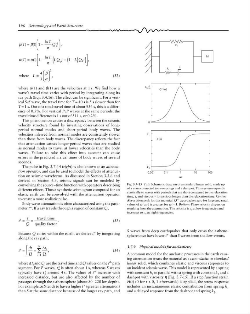
Fig. 3.7-15 Top: Schematic diagram of a standard linear solid, made up
of a mass connected to two springs and a dashpot. This system responds
elastically to waves with periods that are short compared to the relaxation
time, τ, and viscously for periods longer than the relaxation time. Center:
Absorption peak for this material. Q −1 approaches zero for large and small
values of ωτ and is greatest for ωτ = 1. Bottom: Phase velocity dispersion
resulting from the attenuation. The velocity is c 0 at low frequencies and
increases to c ∞ at high frequencies.
β
β
π
µ
( )
( )
ln
,
T
T Q
=
−
⎛
⎝
⎜
⎞
⎠
⎟
−
1 1
1
α
α
π
µ
( )
( )
ln
,
T
T LQ
L Q K
=
−
+ −
( )
(
)
⎡
⎣
⎢
⎢
⎤
⎦
⎥
⎥
−
−
1 1
1
1
1
where L
,
=
⎛
⎝
⎜
⎞
⎠
⎟
4
3
2
β
α
(52)
where α(1) and β(1) are the velocities at 1 s. We find how a
wave’s travel time varies with period by integrating along its
ray path (Eqn 3.4.16). The effect can be significant. For a vertical ScS wave, the travel time for T = 40 s is 5 s slower than for
T = 1 s. Out of a total travel time of about 934 s, this is a difference of 0.5%. For vertical PcP waves at the same periods, the
travel time difference is 1 s out of 511 s, or 0.2%.
This phenomenon causes a discrepancy between the seismic
velocity structure found by inverting observations of longperiod normal modes and short-period body waves. The
velocities inferred from normal modes are consistently slower
than those from body waves. The discrepancy reflects the fact
that attenuation causes longer-period waves that are studied
as normal modes to travel at lower velocities than the body
waves. Failure to take this effect into account can cause
errors in the predicted arrival times of body waves of several
seconds.
The pulse in Fig. 3.7-14 (right) is also known as an attenuation operator, and can be used to model the effects of attenuation on seismic waveforms. As discussed in Section 3.3.6 and
derived in Section 6.3, seismic signals can be modeled by
convolving the source–time function with operators describing
different effects. Thus a synthetic seismogram computed for an
elastic earth can be convolved with the attenuation operator
to create a more realistic pulse.
Body wave attenuation is often characterized using the parameter t*. If a ray travels through a region of constant Q,
t
t
Q
*
.
=
=
travel time
quality factor
(53)
Because Q varies within the earth, we derive t* by integrating
along the ray path,
t
dt
Q
t
Q
i
i
i
N
*
,
=
=
=
∑
Ύ
∆
1
(54)
where ∆t i and Q i are the travel time and Q values on the i th path
segment. For P waves, t* α is often about 1 s, whereas S waves
typically have t* β around 4 s. The values of t* increase with
increased distance, but are also affected by the number of
passages through the asthenosphere (about 80–220 km depth).
For example, ScS tends to have a higher t* (greater attenuation)
than S at the same distance because of the longer ray path, and
S waves from deep earthquakes that only cross the asthenosphere once have lower t* than S waves from shallow events.
3.7.9 Physical models for anelasticity
A common model for the anelastic processes in the earth causing attenuation treats the material as a viscoelastic or standard
linear solid, which combines elastic and viscous responses to
an incident seismic wave. This model is represented by a spring
with constant k 1 in parallel with a spring with constant k 2 and a
dashpot with viscosity η (Fig. 3.7-15). If a step function strain
H(t) (0 for t < 0, 1 afterwards) is applied, the stress response
includes an instantaneous elastic contribution from spring k 1
and a delayed response from the dashpot and spring k 2 ,
0.001
k 1
ωτ
M
k 2
η
Q max
–1
0
C ∞
Q
–1 ( )
ω
C( )
ω
C 0
0.1
1
10
100
Fig. 3.7-15 Top: Schematic diagram of a standard linear solid, made up
of a mass connected to two springs and a dashpot. This system responds
elastically to waves with periods that are short compared to the relaxation
time, τ, and viscously for periods longer than the relaxation time. Center:
Absorption peak for this material. Q −1 approaches zero for large and small
values of ωτ and is greatest for ωτ = 1. Bottom: Phase velocity dispersion
resulting from the attenuation. The velocity is c 0 at low frequencies and
increases to c ∞ at high frequencies.
β
β
π
µ
( )
( )
ln
,
T
T Q
=
−
⎛
⎝
⎜
⎞
⎠
⎟
−
1 1
1
α
α
π
µ
( )
( )
ln
,
T
T LQ
L Q K
=
−
+ −
( )
(
)
⎡
⎣
⎢
⎢
⎤
⎦
⎥
⎥
−
−
1 1
1
1
1
where L
,
=
⎛
⎝
⎜
⎞
⎠
⎟
4
3
2
β
α
(52)
where α(1) and β(1) are the velocities at 1 s. We find how a
wave’s travel time varies with period by integrating along its
ray path (Eqn 3.4.16). The effect can be significant. For a vertical ScS wave, the travel time for T = 40 s is 5 s slower than for
T = 1 s. Out of a total travel time of about 934 s, this is a difference of 0.5%. For vertical PcP waves at the same periods, the
travel time difference is 1 s out of 511 s, or 0.2%.
This phenomenon causes a discrepancy between the seismic
velocity structure found by inverting observations of longperiod normal modes and short-period body waves. The
velocities inferred from normal modes are consistently slower
than those from body waves. The discrepancy reflects the fact
that attenuation causes longer-period waves that are studied
as normal modes to travel at lower velocities than the body
waves. Failure to take this effect into account can cause
errors in the predicted arrival times of body waves of several
seconds.
The pulse in Fig. 3.7-14 (right) is also known as an attenuation operator, and can be used to model the effects of attenuation on seismic waveforms. As discussed in Section 3.3.6 and
derived in Section 6.3, seismic signals can be modeled by
convolving the source–time function with operators describing
different effects. Thus a synthetic seismogram computed for an
elastic earth can be convolved with the attenuation operator
to create a more realistic pulse.
Body wave attenuation is often characterized using the parameter t*. If a ray travels through a region of constant Q,
t
t
Q
*
.
=
=
travel time
quality factor
(53)
Because Q varies within the earth, we derive t* by integrating
along the ray path,
t
dt
Q
t
Q
i
i
i
N
*
,
=
=
=
∑
Ύ
∆
1
(54)
where ∆t i and Q i are the travel time and Q values on the i th path
segment. For P waves, t* α is often about 1 s, whereas S waves
typically have t* β around 4 s. The values of t* increase with
increased distance, but are also affected by the number of
passages through the asthenosphere (about 80–220 km depth).
For example, ScS tends to have a higher t* (greater attenuation)
than S at the same distance because of the longer ray path, and
S waves from deep earthquakes that only cross the asthenosphere once have lower t* than S waves from shallow events.
3.7.9 Physical models for anelasticity
A common model for the anelastic processes in the earth causing attenuation treats the material as a viscoelastic or standard
linear solid, which combines elastic and viscous responses to
an incident seismic wave. This model is represented by a spring
with constant k 1 in parallel with a spring with constant k 2 and a
dashpot with viscosity η (Fig. 3.7-15). If a step function strain
H(t) (0 for t < 0, 1 afterwards) is applied, the stress response
includes an instantaneous elastic contribution from spring k 1
and a delayed response from the dashpot and spring k 2 ,