

3.7 Attenuation and anelasticity 195
t = x/c
Amplitude
t = x/c
t = x/c ∞
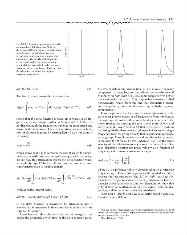
Fig. 3.7-14 Left: A propagating wave pulse
composed of a delta function. With no
dispersion, all frequencies arrive at the same
time. Center: The delta function after
broadening by attenuation, showing that
energy arrives before the high-frequency
arrival time. Right: The pulse including
physical dispersion, which makes the lowerfrequency waves travel more slowly, so that
they do not arrive before the highestfrequency component.
6 We noted a similar effect in Section 2.9.8: namely, that individual normal modes of
a single frequency appear to predict displacement before a wave could arrive, but their
sum gives a wave at the correct time.
7 Aki and Richards (1980).
t = x/c, which is the arrival time of the infinite-frequency
component. In fact, because the tails of the wavelet extend
to infinity on both sides of t = x/c, some energy arrives before
the earthquake occurred. This impossible situation, called
noncausality, results from the fact that attenuation broadened the pulse by preferentially removing the high-frequency
components. 6
Thus the physical mechanisms that cause attenuation in the
earth must prevent waves of all frequencies from traveling at
the same speed. Instead, there must be dispersion, where the
lower frequencies causing the tails travel more slowly and
arrive later. We saw in Section 2.8 that in a dispersive medium
we distinguish the phase velocity c, the speed of a wave of a single
frequency, from the group velocity that describes the speed of a
wave group. Thus the mathematical condition for causality
is that u(x, t) = 0 for all t < x/c ∞ , where c ∞ = c(∞) is the phase
velocity of the infinite-frequency waves that arrive first. One
such dispersion relation for phase velocity as a function of
frequency, called Azimi’s attenuation law, is
c
c
Q
( )
ln
,
ω
π
ω
ω
=
+
⎛
⎝
⎜
⎞
⎠
⎟
⎡
⎣
⎢
⎢
⎤
⎦
⎥
⎥
0
0
1
1
(51)
where c 0 is a reference velocity corresponding to a reference
frequency ω 0 . 7 This relation provides the needed causality,
because the resulting pulse (Fig. 3.7-14, right) has high frequencies arriving at or soon after t = x/c ∞ , whereas the low frequencies arrive later over a duration depending on the value
of Q. If there is no attenuation (Q = ∞), Eqn 51 yields no dispersion, and the delta function is not broadened.
From Eqn 51, the P- and S-wave velocities α and β vary as a
function of period T, as
u(x, t) = δ(t − x/c).
(46)
The Fourier transform of the delta function,
F(ω) =
Ύ
−∞
∞
u(x, t)e −iωt dt =
Ύ
−∞
∞
δ(t − x/c)e −iωt dt = e (−iωx/c) ,
(47)
shows that the delta function is made up of waves of all frequencies, as we discuss further in Section 6.2.5. If there is
no dispersion, all the frequencies travel at the same speed and
arrive at the same time. The effect of attenuation as a function of distance is given by writing Eqn 40 as a function of
frequency,
A
e
x
cQ
( )
,
ω
ω
=
−
2
(48)
which shows that if Q is constant, the rate at which the amplitude decays with distance increases strongly with frequency.
To see how this attenuation affects the delta function wave,
we multiply Eqn 47 by Eqn 48 and use the inverse Fourier
transform to return to the time domain
u(x, t) =
1
2π Ύ
−∞
∞
A(ω)F(ω)e iωt dω =
1
2π Ύ
−∞
∞
e e
x
cQ
i x
c
−
−
ω
ω
2
e iωt dω. (49)
Evaluating the integral yields
u(x, t) = [(x/2cQ)/((x/2cQ) 2 + (x/c − t) 2 )]/π,
(50)
so the delta function is broadened by attenuation into a
wavelet that is symmetric in time about its maximum at t = x/c
(Fig. 3.7-14, center).
A problem with this solution is that seismic energy arrives
before the geometric arrival time of the delta function pulse,
t = x/c
Amplitude
t = x/c
t = x/c ∞
Fig. 3.7-14 Left: A propagating wave pulse
composed of a delta function. With no
dispersion, all frequencies arrive at the same
time. Center: The delta function after
broadening by attenuation, showing that
energy arrives before the high-frequency
arrival time. Right: The pulse including
physical dispersion, which makes the lowerfrequency waves travel more slowly, so that
they do not arrive before the highestfrequency component.
6 We noted a similar effect in Section 2.9.8: namely, that individual normal modes of
a single frequency appear to predict displacement before a wave could arrive, but their
sum gives a wave at the correct time.
7 Aki and Richards (1980).
t = x/c, which is the arrival time of the infinite-frequency
component. In fact, because the tails of the wavelet extend
to infinity on both sides of t = x/c, some energy arrives before
the earthquake occurred. This impossible situation, called
noncausality, results from the fact that attenuation broadened the pulse by preferentially removing the high-frequency
components. 6
Thus the physical mechanisms that cause attenuation in the
earth must prevent waves of all frequencies from traveling at
the same speed. Instead, there must be dispersion, where the
lower frequencies causing the tails travel more slowly and
arrive later. We saw in Section 2.8 that in a dispersive medium
we distinguish the phase velocity c, the speed of a wave of a single
frequency, from the group velocity that describes the speed of a
wave group. Thus the mathematical condition for causality
is that u(x, t) = 0 for all t < x/c ∞ , where c ∞ = c(∞) is the phase
velocity of the infinite-frequency waves that arrive first. One
such dispersion relation for phase velocity as a function of
frequency, called Azimi’s attenuation law, is
c
c
Q
( )
ln
,
ω
π
ω
ω
=
+
⎛
⎝
⎜
⎞
⎠
⎟
⎡
⎣
⎢
⎢
⎤
⎦
⎥
⎥
0
0
1
1
(51)
where c 0 is a reference velocity corresponding to a reference
frequency ω 0 . 7 This relation provides the needed causality,
because the resulting pulse (Fig. 3.7-14, right) has high frequencies arriving at or soon after t = x/c ∞ , whereas the low frequencies arrive later over a duration depending on the value
of Q. If there is no attenuation (Q = ∞), Eqn 51 yields no dispersion, and the delta function is not broadened.
From Eqn 51, the P- and S-wave velocities α and β vary as a
function of period T, as
u(x, t) = δ(t − x/c).
(46)
The Fourier transform of the delta function,
F(ω) =
Ύ
−∞
∞
u(x, t)e −iωt dt =
Ύ
−∞
∞
δ(t − x/c)e −iωt dt = e (−iωx/c) ,
(47)
shows that the delta function is made up of waves of all frequencies, as we discuss further in Section 6.2.5. If there is
no dispersion, all the frequencies travel at the same speed and
arrive at the same time. The effect of attenuation as a function of distance is given by writing Eqn 40 as a function of
frequency,
A
e
x
cQ
( )
,
ω
ω
=
−
2
(48)
which shows that if Q is constant, the rate at which the amplitude decays with distance increases strongly with frequency.
To see how this attenuation affects the delta function wave,
we multiply Eqn 47 by Eqn 48 and use the inverse Fourier
transform to return to the time domain
u(x, t) =
1
2π Ύ
−∞
∞
A(ω)F(ω)e iωt dω =
1
2π Ύ
−∞
∞
e e
x
cQ
i x
c
−
−
ω
ω
2
e iωt dω. (49)
Evaluating the integral yields
u(x, t) = [(x/2cQ)/((x/2cQ) 2 + (x/c − t) 2 )]/π,
(50)
so the delta function is broadened by attenuation into a
wavelet that is symmetric in time about its maximum at t = x/c
(Fig. 3.7-14, center).
A problem with this solution is that seismic energy arrives
before the geometric arrival time of the delta function pulse,