

188 Seismology and Earth Structure
High-velocity region
Actual path
Receiver
Predicted path
Earthquake
Incoming
wave
Amplitudes
Lens
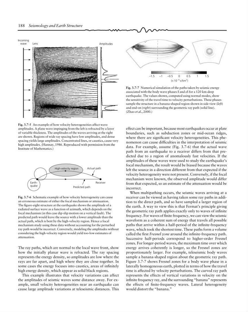
Fig. 3.7-5 An example of how velocity heterogeneities affect wave
amplitudes. A plane wave impinging from the left is refracted by a layer
of variable thickness. The amplitudes of the waves arriving at the right
are shown. Regions of wide ray spacing have low amplitudes, and dense
spacing yields large amplitudes. Concentrated lines, or caustics, cause very
high amplitudes. (Hannay, 1986. Reproduced with permission from the
Institute of Mathematics.)
Fig. 3.7-6 Schematic example of how velocity heterogeneity can cause
an erroneous estimate of either the focal mechanism or attenuation.
The figure-eight structure at the earthquake shows the amplitude of a
radiated surface wave as a function of azimuth, which depends on the
focal mechanism (in this case dip-slip motion on a vertical fault). The
predicted path would leave the source with a lower amplitude than the
actual path, which is bent by the high-velocity region. Hence a focal
mechanism study using these data without accounting for the perturbed
ray path would be incorrect. Conversely, modeling the amplitudes without
considering the high-velocity region would yield too-low estimates of
attenuation.
effect can be important, because most earthquakes occur at plate
boundaries, such as subduction zones or mid-ocean ridges,
where there are significant velocity heterogeneities. This phenomenon can cause difficulties in the interpretation of seismic
data. For example, assume (Fig. 3.7-6) that the actual wave
path from an earthquake to a receiver differs from that predicted due to a region of anomalously fast velocities. If the
amplitudes of these waves were used to study the earthquake’s
focal mechanism, the result would be biased because the waves
left the source in a direction different from that expected if the
velocity heterogeneity were not present. Conversely, if the focal
mechanism were known, the observed amplitude would differ
from that expected, so an estimate of the attenuation would be
incorrect.
When multipathing occurs, the seismic waves arriving at a
receiver can be viewed as having taken some ray paths in addition to the direct path, and so have sampled a larger region of
the earth. A way to view this is that Fermat’s principle giving
the geometric ray path applies exactly only to waves of infinite
frequency. For waves of finite frequency, we can view the seismic
waveform as a coherent sum of energy that travels all possible
paths that arrive within a half-period of the infinite-frequency
wave, which took the shortest time. These paths form a volume
called the first Fresnel zone around the infinite-frequency path.
Successive half-periods correspond to higher-order Fresnel
zones. For longer-period waves, the maximum time over which
energy arrives coherently is longer, so the Fresnel zones are
proportionately larger. For example, teleseismic body waves
sample a banana-shaped region about the geometric ray path.
Figure 3.7-7 shows Fresnel zones for a body wave phase in a
laterally homogeneous earth, plotted in terms of how the travel
time is affected by velocity perturbations. The curved ray path
represents the effects of vertical variations in velocity on the
infinite frequency ray, and the surrounding “banana” represents
the effects of finite-frequency waves. Lateral heterogeneity
would distort the “banana.”
The ray paths, which are normal to the local wave front, show
how the initially planar wave is refracted. The ray spacing
represents the energy density, so amplitudes are low where the
rays are far apart, and high where they are close together. In
some cases the energy focuses into caustics, areas of infinitely
high energy density, which appear as solid black regions.
This example illustrates that velocity variations can affect
the amplitudes of seismic waves some distance away. For example, small velocity heterogeneities near an earthquake can
cause large amplitude variations at teleseismic distances. This
−1.5
(× 10
–6 s/km
3 )
−1
−0.5
0
0.5
1
1.5
Fig. 3.7-7 Numerical simulation of the paths taken by seismic energy
associated with the body wave phases S and sS for a 120 km-deep
earthquake. The values shown, computed using normal modes, show
the sensitivity of the travel time to velocity perturbations. These phases
sample the structure in a banana-shaped region shown in side view (left)
and end-on (right) surrounding the geometric ray path (solid line).
(Zhao et al., 2000.)
High-velocity region
Actual path
Receiver
Predicted path
Earthquake
Incoming
wave
Amplitudes
Lens
Fig. 3.7-5 An example of how velocity heterogeneities affect wave
amplitudes. A plane wave impinging from the left is refracted by a layer
of variable thickness. The amplitudes of the waves arriving at the right
are shown. Regions of wide ray spacing have low amplitudes, and dense
spacing yields large amplitudes. Concentrated lines, or caustics, cause very
high amplitudes. (Hannay, 1986. Reproduced with permission from the
Institute of Mathematics.)
Fig. 3.7-6 Schematic example of how velocity heterogeneity can cause
an erroneous estimate of either the focal mechanism or attenuation.
The figure-eight structure at the earthquake shows the amplitude of a
radiated surface wave as a function of azimuth, which depends on the
focal mechanism (in this case dip-slip motion on a vertical fault). The
predicted path would leave the source with a lower amplitude than the
actual path, which is bent by the high-velocity region. Hence a focal
mechanism study using these data without accounting for the perturbed
ray path would be incorrect. Conversely, modeling the amplitudes without
considering the high-velocity region would yield too-low estimates of
attenuation.
effect can be important, because most earthquakes occur at plate
boundaries, such as subduction zones or mid-ocean ridges,
where there are significant velocity heterogeneities. This phenomenon can cause difficulties in the interpretation of seismic
data. For example, assume (Fig. 3.7-6) that the actual wave
path from an earthquake to a receiver differs from that predicted due to a region of anomalously fast velocities. If the
amplitudes of these waves were used to study the earthquake’s
focal mechanism, the result would be biased because the waves
left the source in a direction different from that expected if the
velocity heterogeneity were not present. Conversely, if the focal
mechanism were known, the observed amplitude would differ
from that expected, so an estimate of the attenuation would be
incorrect.
When multipathing occurs, the seismic waves arriving at a
receiver can be viewed as having taken some ray paths in addition to the direct path, and so have sampled a larger region of
the earth. A way to view this is that Fermat’s principle giving
the geometric ray path applies exactly only to waves of infinite
frequency. For waves of finite frequency, we can view the seismic
waveform as a coherent sum of energy that travels all possible
paths that arrive within a half-period of the infinite-frequency
wave, which took the shortest time. These paths form a volume
called the first Fresnel zone around the infinite-frequency path.
Successive half-periods correspond to higher-order Fresnel
zones. For longer-period waves, the maximum time over which
energy arrives coherently is longer, so the Fresnel zones are
proportionately larger. For example, teleseismic body waves
sample a banana-shaped region about the geometric ray path.
Figure 3.7-7 shows Fresnel zones for a body wave phase in a
laterally homogeneous earth, plotted in terms of how the travel
time is affected by velocity perturbations. The curved ray path
represents the effects of vertical variations in velocity on the
infinite frequency ray, and the surrounding “banana” represents
the effects of finite-frequency waves. Lateral heterogeneity
would distort the “banana.”
The ray paths, which are normal to the local wave front, show
how the initially planar wave is refracted. The ray spacing
represents the energy density, so amplitudes are low where the
rays are far apart, and high where they are close together. In
some cases the energy focuses into caustics, areas of infinitely
high energy density, which appear as solid black regions.
This example illustrates that velocity variations can affect
the amplitudes of seismic waves some distance away. For example, small velocity heterogeneities near an earthquake can
cause large amplitude variations at teleseismic distances. This
−1.5
(× 10
–6 s/km
3 )
−1
−0.5
0
0.5
1
1.5
Fig. 3.7-7 Numerical simulation of the paths taken by seismic energy
associated with the body wave phases S and sS for a 120 km-deep
earthquake. The values shown, computed using normal modes, show
the sensitivity of the travel time to velocity perturbations. These phases
sample the structure in a banana-shaped region shown in side view (left)
and end-on (right) surrounding the geometric ray path (solid line).
(Zhao et al., 2000.)