

182 Seismology and Earth Structure
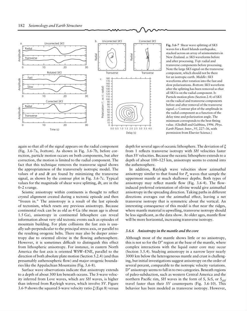
again so that all of the signal appears on the radial component
(Fig. 3.6-7a, bottom). As shown in Fig. 3.6-7b, before correction, particle motion occurs on both components, but after
correction, the motion is limited to the radial component. The
fact that this technique removes the transverse signal shows
the appropriateness of the transversely isotropic model. The
values of φ and δt are found by minimizing the transverse
signal, as shown by the contour plot in Fig. 3.6-7c. Typical
values for the magnitude of shear wave splitting, δt, are in the
0–2 s range.
Seismic anisotropy within continents is thought to reflect
crystal alignment created during a tectonic episode and then
“frozen in.” The anisotropy is a result of the last episode
of tectonism, which resets any previous anisotropy. Because
continental rock can be as old as 4 Ga (the mean age is about
1.5 Ga), anisotropy in continental lithosphere can reveal
information about very old tectonic events such as episodes of
mountain building. For plate collisions the fast axis is usually sub-perpendicular to the principal stress axis, or parallel to
the resulting orogenic belts. There may also be deeper anisotropy due to oriented olivine in the flowing asthenosphere.
However, it is sometimes difficult to distinguish this effect
from lithospheric anisotropy. For instance, in eastern North
America the fast axis is oriented WSW–ENE, parallel to the
direction of both absolute plate motion (Section 5.2.4) (and thus
presumably asthenospheric flow) and major orogenic boundaries like the Appalachian Mountains (Fig. 3.6-8).
Surface wave observations indicate that anisotropy extends
to a depth of about 300 km beneath oceans. The S-wave velocity inferred from Love waves, which are SH waves, is higher
than inferred from Rayleigh waves, which involve SV. Figure
3.6-9 shows the squared S-wave velocity ratio ξ (Eqn 8) versus
depth for several ages of oceanic lithosphere. The deviation of ξ
from 1 reflects transverse isotropy with SH velocities faster
than SV velocities. Because the oceanic lithosphere extends to a
depth of about 100–125 km, anisotropy seems to extend into
the asthenosphere.
In addition, Rayleigh wave velocities show azimuthal
anisotropy similar to that found for P n waves that sample the
uppermost mantle at much shallower depths. Both types of
anisotropy may reflect mantle flow (Fig. 3.6-4). The flowinduced preferred orientation of olivine would give azimuthal
anisotropy in the spreading direction. Taking paths in different
directions averages out the azimuthal effect, leaving a net
transverse isotropy that is symmetric about the vertical. An
interesting consequence of this model is that near the ridges,
where mantle material is upwelling, transverse isotropy should
be less significant, as the data show. At older ages, mantle flow
will be more horizontal, increasing transverse isotropy.
3.6.6 Anisotropy in the mantle and the core
Although most of the mantle shows little or no anisotropy,
this is not so for the D″ region at the base of the mantle, where
complex interactions with the liquid outer core may occur
(Section 3.5.4). Studying anisotropy in a narrow layer nearly
3000 km below the heterogeneous mantle and crust is challenging, but initial investigations suggest anisotropy on the order of
several percent, comparable to the isotropic velocity variations.
D″ anisotropy seems to fall in to two categories. Beneath regions
of paleo-subduction, such as western Central America and the
northern Pacific rim, SH waves in the form of S, ScS, or S diff
travel faster than their SV counterparts (Fig. 3.6-10). This
behavior has been modeled as transverse isotropy. However,
Amplitude
Uncorrected SKS
Radial
Transverse
Fast
Slow
Radial
Transverse
Time (s)
Delay (s)
c.
b.
a.
Transverse
Transverse
Uncorrected SKS
Rotated SKS
Corrected SKS
Corrected SKS
0
Radial
Radial
Polarization (°, w.r.t. radial)
180
170
160
150
140
130
120
110
100
90
80
70
60
50
40
30
20
10
0
10
20
30
Amplitude
0
10
20
30
Amplitude
0
10
20
30
4
6
4
0.5
0.0
1.5
1.0
2.5
2.0
3.5
3.0
4.0
Fig. 3.6-7 Shear wave splitting of SKS
waves for a Kuril Islands earthquake,
stacked across an array of seismometers in
New Zealand. a: SKS waveforms before
and after processing. Top: radial and
transverse components before processing.
Note the large SKS signal on the transverse
component, which should not be there
for an isotropic earth. Middle: SKS
waveforms after rotation into the fast and
slow polarizations. Bottom: SKS waveform
after the splitting has been removed so that
all SKS is on the radial component. b:
Particle motion plots (Section 2.4) of SKS
on the radical and transverse components
before and after removal of the transverse
signal. c: Contour plot of the amplitude in
the radial component as a function of the
delay time and polarization angle. The
minimum corresponds to the best-fitting
value. (Gledhill and Gubbins, 1996. Phys.
Earth Planet. Inter., 95, 227–36, with
permission from Elsevier Science.)
again so that all of the signal appears on the radial component
(Fig. 3.6-7a, bottom). As shown in Fig. 3.6-7b, before correction, particle motion occurs on both components, but after
correction, the motion is limited to the radial component. The
fact that this technique removes the transverse signal shows
the appropriateness of the transversely isotropic model. The
values of φ and δt are found by minimizing the transverse
signal, as shown by the contour plot in Fig. 3.6-7c. Typical
values for the magnitude of shear wave splitting, δt, are in the
0–2 s range.
Seismic anisotropy within continents is thought to reflect
crystal alignment created during a tectonic episode and then
“frozen in.” The anisotropy is a result of the last episode
of tectonism, which resets any previous anisotropy. Because
continental rock can be as old as 4 Ga (the mean age is about
1.5 Ga), anisotropy in continental lithosphere can reveal
information about very old tectonic events such as episodes of
mountain building. For plate collisions the fast axis is usually sub-perpendicular to the principal stress axis, or parallel to
the resulting orogenic belts. There may also be deeper anisotropy due to oriented olivine in the flowing asthenosphere.
However, it is sometimes difficult to distinguish this effect
from lithospheric anisotropy. For instance, in eastern North
America the fast axis is oriented WSW–ENE, parallel to the
direction of both absolute plate motion (Section 5.2.4) (and thus
presumably asthenospheric flow) and major orogenic boundaries like the Appalachian Mountains (Fig. 3.6-8).
Surface wave observations indicate that anisotropy extends
to a depth of about 300 km beneath oceans. The S-wave velocity inferred from Love waves, which are SH waves, is higher
than inferred from Rayleigh waves, which involve SV. Figure
3.6-9 shows the squared S-wave velocity ratio ξ (Eqn 8) versus
depth for several ages of oceanic lithosphere. The deviation of ξ
from 1 reflects transverse isotropy with SH velocities faster
than SV velocities. Because the oceanic lithosphere extends to a
depth of about 100–125 km, anisotropy seems to extend into
the asthenosphere.
In addition, Rayleigh wave velocities show azimuthal
anisotropy similar to that found for P n waves that sample the
uppermost mantle at much shallower depths. Both types of
anisotropy may reflect mantle flow (Fig. 3.6-4). The flowinduced preferred orientation of olivine would give azimuthal
anisotropy in the spreading direction. Taking paths in different
directions averages out the azimuthal effect, leaving a net
transverse isotropy that is symmetric about the vertical. An
interesting consequence of this model is that near the ridges,
where mantle material is upwelling, transverse isotropy should
be less significant, as the data show. At older ages, mantle flow
will be more horizontal, increasing transverse isotropy.
3.6.6 Anisotropy in the mantle and the core
Although most of the mantle shows little or no anisotropy,
this is not so for the D″ region at the base of the mantle, where
complex interactions with the liquid outer core may occur
(Section 3.5.4). Studying anisotropy in a narrow layer nearly
3000 km below the heterogeneous mantle and crust is challenging, but initial investigations suggest anisotropy on the order of
several percent, comparable to the isotropic velocity variations.
D″ anisotropy seems to fall in to two categories. Beneath regions
of paleo-subduction, such as western Central America and the
northern Pacific rim, SH waves in the form of S, ScS, or S diff
travel faster than their SV counterparts (Fig. 3.6-10). This
behavior has been modeled as transverse isotropy. However,
Amplitude
Uncorrected SKS
Radial
Transverse
Fast
Slow
Radial
Transverse
Time (s)
Delay (s)
c.
b.
a.
Transverse
Transverse
Uncorrected SKS
Rotated SKS
Corrected SKS
Corrected SKS
0
Radial
Radial
Polarization (°, w.r.t. radial)
180
170
160
150
140
130
120
110
100
90
80
70
60
50
40
30
20
10
0
10
20
30
Amplitude
0
10
20
30
Amplitude
0
10
20
30
4
6
4
0.5
0.0
1.5
1.0
2.5
2.0
3.5
3.0
4.0
Fig. 3.6-7 Shear wave splitting of SKS
waves for a Kuril Islands earthquake,
stacked across an array of seismometers in
New Zealand. a: SKS waveforms before
and after processing. Top: radial and
transverse components before processing.
Note the large SKS signal on the transverse
component, which should not be there
for an isotropic earth. Middle: SKS
waveforms after rotation into the fast and
slow polarizations. Bottom: SKS waveform
after the splitting has been removed so that
all SKS is on the radial component. b:
Particle motion plots (Section 2.4) of SKS
on the radical and transverse components
before and after removal of the transverse
signal. c: Contour plot of the amplitude in
the radial component as a function of the
delay time and polarization angle. The
minimum corresponds to the best-fitting
value. (Gledhill and Gubbins, 1996. Phys.
Earth Planet. Inter., 95, 227–36, with
permission from Elsevier Science.)