

cover
mid-crustal mylonite
zone related to
thrust belt compression
possible gabbroic
intrusions largely
sheared and rotated
large scale pure shear
accommodated by simple
shear concentrated on
lower crustal mylonite zones
mafic cumulate or residuum
Moho, consisting of
interlayered mantle
and crustal rocks —
possible magma
Eromanga basin
No reflections
Mid — crustal boundary
Lower crustal reflections
Moho
Upper mantle
0
10 km
detachment fault
mylonite zone
migmatitic core
E
W
M
(Fig. 3.6-4, top) appear to orient olivine crystals preferentially
in the spreading direction, along their [100] slip axes. 1 Because
P waves propagate fastest in this direction (Fig. 3.6-3), P n head
waves that sample the uppermost mantle just below the Moho
(Section 3.2.1) show a strong azimuthal velocity dependence
(Fig. 3.6-4, bottom). This variation is approximately described
by the cos 2θ term in Eqn 9, where θ is measured from the
spreading direction, so the velocity is highest in the spreading
direction or 180° from it. This anisotropy is “frozen in” as the
lithosphere ages, and so records the spreading direction.
Because continental crust is more complicated than oceanic
crust, so is its anisotropy. A primary source of anisotropy in
the upper crust is the presence of cracks, often fluid-filled.
Such cracks often have a near-vertical orientation induced by
regional stress fields parallel to the cracks. When these cracks
occur in horizontal sediments that would by themselves have
vertical-axis transverse isotropy, the combined result can be
orthorhombic symmetry. The lower continental crust tends to
have strong sub-horizontal layering, perhaps resulting from
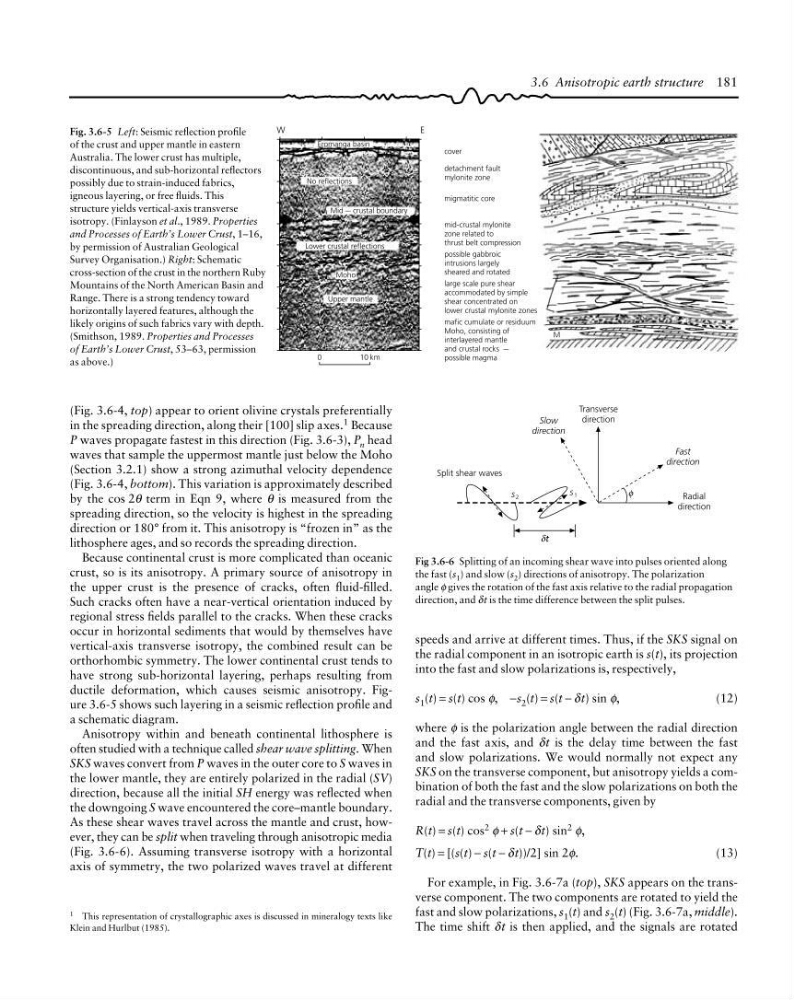
ductile deformation, which causes seismic anisotropy. Figure 3.6-5 shows such layering in a seismic reflection profile and
a schematic diagram.
Anisotropy within and beneath continental lithosphere is
often studied with a technique called shear wave splitting. When
SKS waves convert from P waves in the outer core to S waves in
the lower mantle, they are entirely polarized in the radial (SV)
direction, because all the initial SH energy was reflected when
the downgoing S wave encountered the core–mantle boundary.
As these shear waves travel across the mantle and crust, however, they can be split when traveling through anisotropic media
(Fig. 3.6-6). Assuming transverse isotropy with a horizontal
axis of symmetry, the two polarized waves travel at different
3.6 Anisotropic earth structure 181
1 This representation of crystallographic axes is discussed in mineralogy texts like
Klein and Hurlbut (1985).
Fig. 3.6-5 Left: Seismic reflection profile
of the crust and upper mantle in eastern
Australia. The lower crust has multiple,
discontinuous, and sub-horizontal reflectors
possibly due to strain-induced fabrics,
igneous layering, or free fluids. This
structure yields vertical-axis transverse
isotropy. (Finlayson et al., 1989. Properties
and Processes of Earth’s Lower Crust, 1–16,
by permission of Australian Geological
Survey Organisation.) Right: Schematic
cross-section of the crust in the northern Ruby
Mountains of the North American Basin and
Range. There is a strong tendency toward
horizontally layered features, although the
likely origins of such fabrics vary with depth.
(Smithson, 1989. Properties and Processes
of Earth’s Lower Crust, 53–63, permission
as above.)
Transverse
direction
Radial
direction
Split shear waves
φ
Slow
direction
s 2
s 1
Fast
direction
t
δ
Fig 3.6-6 Splitting of an incoming shear wave into pulses oriented along
the fast (s 1 ) and slow (s 2 ) directions of anisotropy. The polarization
angle φ gives the rotation of the fast axis relative to the radial propagation
direction, and δt is the time difference between the split pulses.
speeds and arrive at different times. Thus, if the SKS signal on
the radial component in an isotropic earth is s(t), its projection
into the fast and slow polarizations is, respectively,
s 1 (t) = s(t) cos φ, −s 2 (t) = s(t − δt) sin φ,
(12)
where φ is the polarization angle between the radial direction
and the fast axis, and δt is the delay time between the fast
and slow polarizations. We would normally not expect any
SKS on the transverse component, but anisotropy yields a combination of both the fast and the slow polarizations on both the
radial and the transverse components, given by
R(t) = s(t) cos 2 φ + s(t − δt) sin 2 φ,
T(t) = [(s(t) − s(t − δt))/2] sin 2φ.
(13)
For example, in Fig. 3.6-7a (top), SKS appears on the transverse component. The two components are rotated to yield the
fast and slow polarizations, s 1 (t) and s 2 (t) (Fig. 3.6-7a, middle).
The time shift δt is then applied, and the signals are rotated
mid-crustal mylonite
zone related to
thrust belt compression
possible gabbroic
intrusions largely
sheared and rotated
large scale pure shear
accommodated by simple
shear concentrated on
lower crustal mylonite zones
mafic cumulate or residuum
Moho, consisting of
interlayered mantle
and crustal rocks —
possible magma
Eromanga basin
No reflections
Mid — crustal boundary
Lower crustal reflections
Moho
Upper mantle
0
10 km
detachment fault
mylonite zone
migmatitic core
E
W
M
(Fig. 3.6-4, top) appear to orient olivine crystals preferentially
in the spreading direction, along their [100] slip axes. 1 Because
P waves propagate fastest in this direction (Fig. 3.6-3), P n head
waves that sample the uppermost mantle just below the Moho
(Section 3.2.1) show a strong azimuthal velocity dependence
(Fig. 3.6-4, bottom). This variation is approximately described
by the cos 2θ term in Eqn 9, where θ is measured from the
spreading direction, so the velocity is highest in the spreading
direction or 180° from it. This anisotropy is “frozen in” as the
lithosphere ages, and so records the spreading direction.
Because continental crust is more complicated than oceanic
crust, so is its anisotropy. A primary source of anisotropy in
the upper crust is the presence of cracks, often fluid-filled.
Such cracks often have a near-vertical orientation induced by
regional stress fields parallel to the cracks. When these cracks
occur in horizontal sediments that would by themselves have
vertical-axis transverse isotropy, the combined result can be
orthorhombic symmetry. The lower continental crust tends to
have strong sub-horizontal layering, perhaps resulting from
ductile deformation, which causes seismic anisotropy. Figure 3.6-5 shows such layering in a seismic reflection profile and
a schematic diagram.
Anisotropy within and beneath continental lithosphere is
often studied with a technique called shear wave splitting. When
SKS waves convert from P waves in the outer core to S waves in
the lower mantle, they are entirely polarized in the radial (SV)
direction, because all the initial SH energy was reflected when
the downgoing S wave encountered the core–mantle boundary.
As these shear waves travel across the mantle and crust, however, they can be split when traveling through anisotropic media
(Fig. 3.6-6). Assuming transverse isotropy with a horizontal
axis of symmetry, the two polarized waves travel at different
3.6 Anisotropic earth structure 181
1 This representation of crystallographic axes is discussed in mineralogy texts like
Klein and Hurlbut (1985).
Fig. 3.6-5 Left: Seismic reflection profile
of the crust and upper mantle in eastern
Australia. The lower crust has multiple,
discontinuous, and sub-horizontal reflectors
possibly due to strain-induced fabrics,
igneous layering, or free fluids. This
structure yields vertical-axis transverse
isotropy. (Finlayson et al., 1989. Properties
and Processes of Earth’s Lower Crust, 1–16,
by permission of Australian Geological
Survey Organisation.) Right: Schematic
cross-section of the crust in the northern Ruby
Mountains of the North American Basin and
Range. There is a strong tendency toward
horizontally layered features, although the
likely origins of such fabrics vary with depth.
(Smithson, 1989. Properties and Processes
of Earth’s Lower Crust, 53–63, permission
as above.)
Transverse
direction
Radial
direction
Split shear waves
φ
Slow
direction
s 2
s 1
Fast
direction
t
δ
Fig 3.6-6 Splitting of an incoming shear wave into pulses oriented along
the fast (s 1 ) and slow (s 2 ) directions of anisotropy. The polarization
angle φ gives the rotation of the fast axis relative to the radial propagation
direction, and δt is the time difference between the split pulses.
speeds and arrive at different times. Thus, if the SKS signal on
the radial component in an isotropic earth is s(t), its projection
into the fast and slow polarizations is, respectively,
s 1 (t) = s(t) cos φ, −s 2 (t) = s(t − δt) sin φ,
(12)
where φ is the polarization angle between the radial direction
and the fast axis, and δt is the delay time between the fast
and slow polarizations. We would normally not expect any
SKS on the transverse component, but anisotropy yields a combination of both the fast and the slow polarizations on both the
radial and the transverse components, given by
R(t) = s(t) cos 2 φ + s(t − δt) sin 2 φ,
T(t) = [(s(t) − s(t − δt))/2] sin 2φ.
(13)
For example, in Fig. 3.6-7a (top), SKS appears on the transverse component. The two components are rotated to yield the
fast and slow polarizations, s 1 (t) and s 2 (t) (Fig. 3.6-7a, middle).
The time shift δt is then applied, and the signals are rotated