

178 Seismology and Earth Structure
For an isotropic material, the c ijkl tensor can be written in terms
of two independent elastic constants
c ijkl = λδ ij δ kl + µ(δ ik δ jl + δ il δ jk ),
(3)
so its matrix form is
C mn =
+
+
+
⎛
⎝
⎜
⎜
⎜
⎜
⎜
⎜ ⎜
⎞
⎠
⎟
⎟
⎟
⎟
⎟
⎟ ⎟
.
λ
µ
λ
λ
λ
λ
µ
λ
λ
λ
λ
µ
µ
µ
µ
2
0 0 0
2
0 0 0
2
0 0 0
0
0
0
0 0
0
0
0
0
0
0
0
0
0 0
(4)
However, the crystal structures of many earth materials require additional independent elastic coefficients. For example,
ice, quartz, olivine, or plagioclase feldspar require 5, 6, 9, and
21 constants, respectively. In such cases, the matrix is more
complicated.
One of the most important forms of anisotropy, known
as transverse isotropy (also known as radial anisotropy,
axisymmetry, and cylindrical symmetry), occurs for a stack of
layered materials. Each layer is isotropic in its properties, but
these properties differ between layers (as in plywood). Thus the
elastic properties, and hence seismic velocities, of the stack as
a whole are identical regardless of the amount of rotation
about the axis of symmetry, which is perpendicular to the layers.
However, these aggregate properties differ in the perpendicular
directions.
A transversely isotropic material can be characterized by five
independent elastic coefficients, A, C, F, L, N, that represent its
aggregate properties. If the axis of symmetry is x 3 , so properties
in that direction differ from those in the x 1 –x 2 plane, the elastic
constant matrix (Eqn 4) becomes
C
A
A
N F
A
N
A
F
F
F
C
L
L
N
mn =
−
−
⎛
⎝
⎜
⎜
⎜
⎜
⎜
⎜
⎞
⎠
⎟
⎟
⎟
⎟
⎟
⎟
.
2
0 0 0
2
0 0 0
0 0 0
0
0
0
0 0
0
0
0 0
0
0
0
0 0 0
(5)
Comparisons with matrices 2 and 4 show that terms that were
the same for an isotropic material (consider C 11 and C 33 , or C 55
and C 66 ) now differ, because terms involving the x 3 direction
differ from those in the x 1 or x 2 directions.
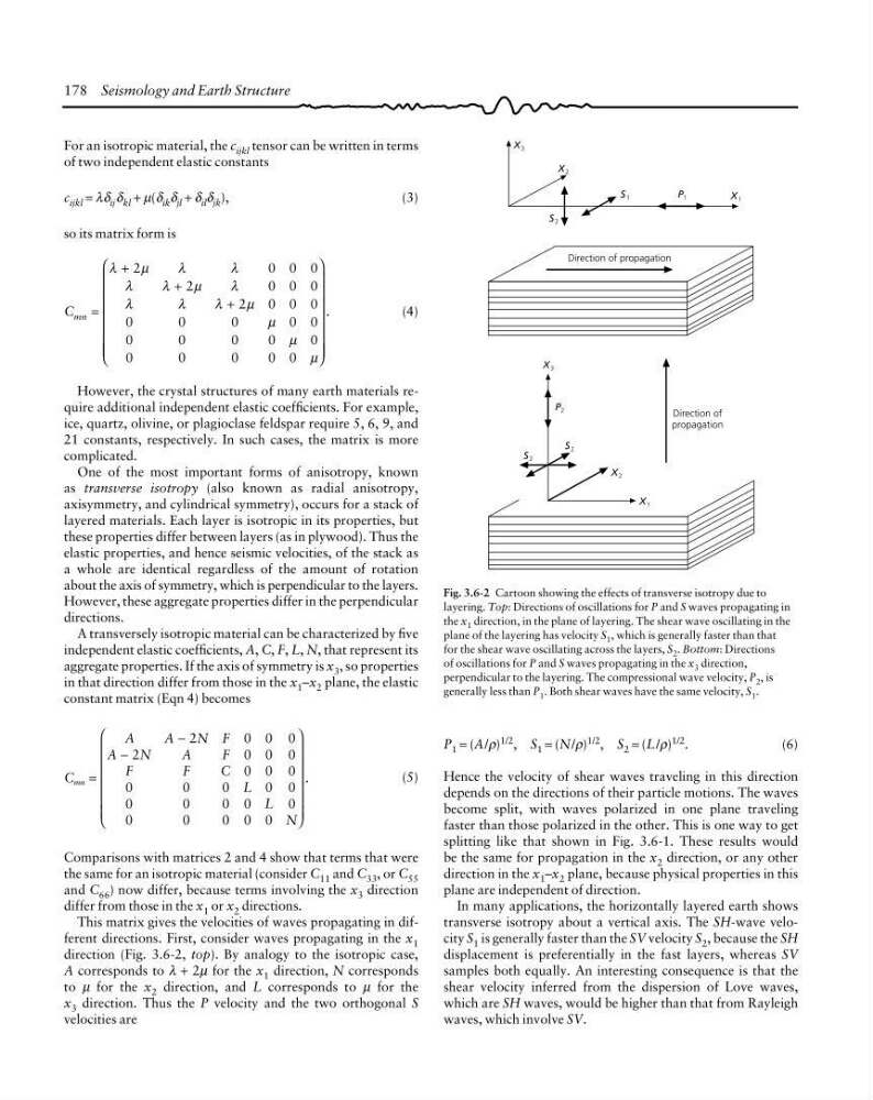
This matrix gives the velocities of waves propagating in different directions. First, consider waves propagating in the x 1
direction (Fig. 3.6-2, top). By analogy to the isotropic case,
A corresponds to λ + 2µ for the x 1 direction, N corresponds
to µ for the x 2 direction, and L corresponds to µ for the
x 3 direction. Thus the P velocity and the two orthogonal S
velocities are
P 1 = (A/ρ) 1/2 , S 1 = (N/ρ) 1/2 , S 2 = (L/ρ) 1/2 .
(6)
Hence the velocity of shear waves traveling in this direction
depends on the directions of their particle motions. The waves
become split, with waves polarized in one plane traveling
faster than those polarized in the other. This is one way to get
splitting like that shown in Fig. 3.6-1. These results would
be the same for propagation in the x 2 direction, or any other
direction in the x 1 –x 2 plane, because physical properties in this
plane are independent of direction.
In many applications, the horizontally layered earth shows
transverse isotropy about a vertical axis. The SH-wave velocity S 1 is generally faster than the SV velocity S 2 , because the SH
displacement is preferentially in the fast layers, whereas SV
samples both equally. An interesting consequence is that the
shear velocity inferred from the dispersion of Love waves,
which are SH waves, would be higher than that from Rayleigh
waves, which involve SV.
Direction of propagation
S 2
S 1
P 1
X 1
X 3
X 3
P 2
S 2
S 2
X 2
X 1
Direction of
propagation
X 2
Fig. 3.6-2 Cartoon showing the effects of transverse isotropy due to
layering. Top: Directions of oscillations for P and S waves propagating in
the x 1 direction, in the plane of layering. The shear wave oscillating in the
plane of the layering has velocity S 1 , which is generally faster than that
for the shear wave oscillating across the layers, S 2 . Bottom: Directions
of oscillations for P and S waves propagating in the x 3 direction,
perpendicular to the layering. The compressional wave velocity, P 2 , is
generally less than P 1 . Both shear waves have the same velocity, S 1 .
For an isotropic material, the c ijkl tensor can be written in terms
of two independent elastic constants
c ijkl = λδ ij δ kl + µ(δ ik δ jl + δ il δ jk ),
(3)
so its matrix form is
C mn =
+
+
+
⎛
⎝
⎜
⎜
⎜
⎜
⎜
⎜ ⎜
⎞
⎠
⎟
⎟
⎟
⎟
⎟
⎟ ⎟
.
λ
µ
λ
λ
λ
λ
µ
λ
λ
λ
λ
µ
µ
µ
µ
2
0 0 0
2
0 0 0
2
0 0 0
0
0
0
0 0
0
0
0
0
0
0
0
0
0 0
(4)
However, the crystal structures of many earth materials require additional independent elastic coefficients. For example,
ice, quartz, olivine, or plagioclase feldspar require 5, 6, 9, and
21 constants, respectively. In such cases, the matrix is more
complicated.
One of the most important forms of anisotropy, known
as transverse isotropy (also known as radial anisotropy,
axisymmetry, and cylindrical symmetry), occurs for a stack of
layered materials. Each layer is isotropic in its properties, but
these properties differ between layers (as in plywood). Thus the
elastic properties, and hence seismic velocities, of the stack as
a whole are identical regardless of the amount of rotation
about the axis of symmetry, which is perpendicular to the layers.
However, these aggregate properties differ in the perpendicular
directions.
A transversely isotropic material can be characterized by five
independent elastic coefficients, A, C, F, L, N, that represent its
aggregate properties. If the axis of symmetry is x 3 , so properties
in that direction differ from those in the x 1 –x 2 plane, the elastic
constant matrix (Eqn 4) becomes
C
A
A
N F
A
N
A
F
F
F
C
L
L
N
mn =
−
−
⎛
⎝
⎜
⎜
⎜
⎜
⎜
⎜
⎞
⎠
⎟
⎟
⎟
⎟
⎟
⎟
.
2
0 0 0
2
0 0 0
0 0 0
0
0
0
0 0
0
0
0 0
0
0
0
0 0 0
(5)
Comparisons with matrices 2 and 4 show that terms that were
the same for an isotropic material (consider C 11 and C 33 , or C 55
and C 66 ) now differ, because terms involving the x 3 direction
differ from those in the x 1 or x 2 directions.
This matrix gives the velocities of waves propagating in different directions. First, consider waves propagating in the x 1
direction (Fig. 3.6-2, top). By analogy to the isotropic case,
A corresponds to λ + 2µ for the x 1 direction, N corresponds
to µ for the x 2 direction, and L corresponds to µ for the
x 3 direction. Thus the P velocity and the two orthogonal S
velocities are
P 1 = (A/ρ) 1/2 , S 1 = (N/ρ) 1/2 , S 2 = (L/ρ) 1/2 .
(6)
Hence the velocity of shear waves traveling in this direction
depends on the directions of their particle motions. The waves
become split, with waves polarized in one plane traveling
faster than those polarized in the other. This is one way to get
splitting like that shown in Fig. 3.6-1. These results would
be the same for propagation in the x 2 direction, or any other
direction in the x 1 –x 2 plane, because physical properties in this
plane are independent of direction.
In many applications, the horizontally layered earth shows
transverse isotropy about a vertical axis. The SH-wave velocity S 1 is generally faster than the SV velocity S 2 , because the SH
displacement is preferentially in the fast layers, whereas SV
samples both equally. An interesting consequence is that the
shear velocity inferred from the dispersion of Love waves,
which are SH waves, would be higher than that from Rayleigh
waves, which involve SV.
Direction of propagation
S 2
S 1
P 1
X 1
X 3
X 3
P 2
S 2
S 2
X 2
X 1
Direction of
propagation
X 2
Fig. 3.6-2 Cartoon showing the effects of transverse isotropy due to
layering. Top: Directions of oscillations for P and S waves propagating in
the x 1 direction, in the plane of layering. The shear wave oscillating in the
plane of the layering has velocity S 1 , which is generally faster than that
for the shear wave oscillating across the layers, S 2 . Bottom: Directions
of oscillations for P and S waves propagating in the x 3 direction,
perpendicular to the layering. The compressional wave velocity, P 2 , is
generally less than P 1 . Both shear waves have the same velocity, S 1 .