

3.6 Anisotropic earth structure
3.6.1 General considerations
So far in this chapter, we have considered a view of the earth
developed from analyses of seismic waves assuming that they
propagated through an earth made up of purely isotropic,
linearly elastic material (Section 2.3.9). In such material, the
stresses are linearly proportional to the strains via Hooke’s law
σ ij = c ijkl e kl ,
(1)
and the 81-term tensor of elastic moduli, c ijkl , reduces to two
independent elastic constants, λ and µ. As a result, the material’s
elastic properties are the same in all directions. Although isotropy is a good first approximation in the earth, it is sometimes
important to consider deviations from isotropy, or anisotropy.
In such cases, Hooke’s law applies, but the relation between the
stresses and strains involves more than two elastic constants.
Although there can be up to 21 independent elastic constants,
any material in which more than two are needed is called
anisotropic.
Having more than two elastic constants means that the
material’s properties differ depending on the direction. Because
seismic wave velocities depend on the elastic constants, waves
traveling through anisotropic material travel faster or slower
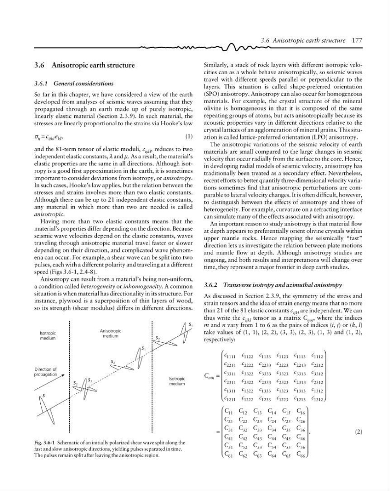
depending on their direction, and complicated wave phenomena can occur. For example, a shear wave can be split into two
pulses, each with a different polarity and traveling at a different
speed (Figs 3.6-1, 2.4-8).
Anisotropy can result from a material’s being non-uniform,
a condition called heterogeneity or inhomogeneity. A common
situation is when material has directionality in its structure. For
instance, plywood is a superposition of thin layers of wood,
so its strength (shear modulus) differs in different directions.
Similarly, a stack of rock layers with different isotropic velocities can as a whole behave anisotropically, so seismic waves
travel with different speeds parallel or perpendicular to the
layers. This situation is called shape-preferred orientation
(SPO) anisotropy. Anisotropy can also occur for homogeneous
materials. For example, the crystal structure of the mineral
olivine is homogeneous in that it is composed of the same
repeating groups of atoms, but acts anisotropically because its
acoustic properties vary in different directions relative to the
crystal lattices of an agglomeration of mineral grains. This situation is called lattice-preferred orientation (LPO) anisotropy.
The anisotropic variations of the seismic velocity of earth
materials are small compared to the large changes in seismic
velocity that occur radially from the surface to the core. Hence,
in developing radial models of seismic velocity, anisotropy has
traditionally been treated as a secondary effect. Nevertheless,
recent efforts to better quantify three-dimensional velocity variations sometimes find that anisotropic perturbations are comparable to lateral velocity changes. It is often difficult, however,
to distinguish between the effects of anisotropy and those of
heterogeneity. For example, curvature on a refracting interface
can simulate many of the effects associated with anisotropy.
An important reason to study anisotropy is that material flow
at depth appears to preferentially orient olivine crystals within
upper mantle rocks. Hence mapping the seismically “fast”
direction lets us investigate the relation between plate motions
and mantle flow at depth. Although anisotropy studies are
ongoing, and both results and interpretations will change over
time, they represent a major frontier in deep earth studies.
3.6.2 Transverse isotropy and azimuthal anisotropy
As discussed in Section 2.3.9, the symmetry of the stress and
strain tensors and the idea of strain energy means that no more
than 21 of the 81 elastic constants c ijkl are independent. We can
thus write the c ijkl tensor as a matrix C mn , where the indices
m and n vary from 1 to 6 as the pairs of indices (i, j) or (k, l)
take values of (1, 1), (2, 2), (3, 3), (2, 3), (1, 3) and (1, 2),
respectively:
C
c
c
c
c
c
c
c
c
c
c
c
c
c
c
c
c
c
c
c
c
c
c
c
c
c
c
c
c
c
c
c
c
c
c
c
c
mn =
⎛
⎝
⎜
⎜
⎜
⎜
⎜
⎜
⎜
⎞
⎠
⎟
⎟
⎟
⎟
⎟
⎟
⎟
1111
1122
1133
1123
1113
1112
2211
2222
2233
2223
2213
2212
3311
3322
3333
3323
3313
3312
2311
2322
2333
2323
2313
2312
1311
1322
1333
1323
1313
1312
1211
1222
1233
1223
1213
1212
=
⎛
⎝
⎜
⎜
⎜
⎜
⎜
⎜
⎜
⎞
⎠
⎟
⎟
⎟
⎟
⎟
⎟
⎟
.
C
C
C
C
C
C
C
C
C
C
C
C
C
C
C
C
C
C
C
C
C
C
C
C
C
C
C
C
C
C
C
C
C
C
C
C
11
12
13
14
15
16
21
22
23
24
25
26
31
32
33
34
35
36
41
42
43
44
45
46
51
52
53
54
55
56
61
62
63
64
65
66
(2)
3.6 Anisotropic earth structure 177
Fig. 3.6-1 Schematic of an initially polarized shear wave split along the
fast and slow anisotropic directions, yielding pulses separated in time.
The pulses remain split after leaving the anisotropic region.
Direction of
propagation
Isotropic
medium
Anisotropic
medium
Isotropic
medium
S
S 2
S 2
S 1
S 1
S 1
S 2
3.6.1 General considerations
So far in this chapter, we have considered a view of the earth
developed from analyses of seismic waves assuming that they
propagated through an earth made up of purely isotropic,
linearly elastic material (Section 2.3.9). In such material, the
stresses are linearly proportional to the strains via Hooke’s law
σ ij = c ijkl e kl ,
(1)
and the 81-term tensor of elastic moduli, c ijkl , reduces to two
independent elastic constants, λ and µ. As a result, the material’s
elastic properties are the same in all directions. Although isotropy is a good first approximation in the earth, it is sometimes
important to consider deviations from isotropy, or anisotropy.
In such cases, Hooke’s law applies, but the relation between the
stresses and strains involves more than two elastic constants.
Although there can be up to 21 independent elastic constants,
any material in which more than two are needed is called
anisotropic.
Having more than two elastic constants means that the
material’s properties differ depending on the direction. Because
seismic wave velocities depend on the elastic constants, waves
traveling through anisotropic material travel faster or slower
depending on their direction, and complicated wave phenomena can occur. For example, a shear wave can be split into two
pulses, each with a different polarity and traveling at a different
speed (Figs 3.6-1, 2.4-8).
Anisotropy can result from a material’s being non-uniform,
a condition called heterogeneity or inhomogeneity. A common
situation is when material has directionality in its structure. For
instance, plywood is a superposition of thin layers of wood,
so its strength (shear modulus) differs in different directions.
Similarly, a stack of rock layers with different isotropic velocities can as a whole behave anisotropically, so seismic waves
travel with different speeds parallel or perpendicular to the
layers. This situation is called shape-preferred orientation
(SPO) anisotropy. Anisotropy can also occur for homogeneous
materials. For example, the crystal structure of the mineral
olivine is homogeneous in that it is composed of the same
repeating groups of atoms, but acts anisotropically because its
acoustic properties vary in different directions relative to the
crystal lattices of an agglomeration of mineral grains. This situation is called lattice-preferred orientation (LPO) anisotropy.
The anisotropic variations of the seismic velocity of earth
materials are small compared to the large changes in seismic
velocity that occur radially from the surface to the core. Hence,
in developing radial models of seismic velocity, anisotropy has
traditionally been treated as a secondary effect. Nevertheless,
recent efforts to better quantify three-dimensional velocity variations sometimes find that anisotropic perturbations are comparable to lateral velocity changes. It is often difficult, however,
to distinguish between the effects of anisotropy and those of
heterogeneity. For example, curvature on a refracting interface
can simulate many of the effects associated with anisotropy.
An important reason to study anisotropy is that material flow
at depth appears to preferentially orient olivine crystals within
upper mantle rocks. Hence mapping the seismically “fast”
direction lets us investigate the relation between plate motions
and mantle flow at depth. Although anisotropy studies are
ongoing, and both results and interpretations will change over
time, they represent a major frontier in deep earth studies.
3.6.2 Transverse isotropy and azimuthal anisotropy
As discussed in Section 2.3.9, the symmetry of the stress and
strain tensors and the idea of strain energy means that no more
than 21 of the 81 elastic constants c ijkl are independent. We can
thus write the c ijkl tensor as a matrix C mn , where the indices
m and n vary from 1 to 6 as the pairs of indices (i, j) or (k, l)
take values of (1, 1), (2, 2), (3, 3), (2, 3), (1, 3) and (1, 2),
respectively:
C
c
c
c
c
c
c
c
c
c
c
c
c
c
c
c
c
c
c
c
c
c
c
c
c
c
c
c
c
c
c
c
c
c
c
c
c
mn =
⎛
⎝
⎜
⎜
⎜
⎜
⎜
⎜
⎜
⎞
⎠
⎟
⎟
⎟
⎟
⎟
⎟
⎟
1111
1122
1133
1123
1113
1112
2211
2222
2233
2223
2213
2212
3311
3322
3333
3323
3313
3312
2311
2322
2333
2323
2313
2312
1311
1322
1333
1323
1313
1312
1211
1222
1233
1223
1213
1212
=
⎛
⎝
⎜
⎜
⎜
⎜
⎜
⎜
⎜
⎞
⎠
⎟
⎟
⎟
⎟
⎟
⎟
⎟
.
C
C
C
C
C
C
C
C
C
C
C
C
C
C
C
C
C
C
C
C
C
C
C
C
C
C
C
C
C
C
C
C
C
C
C
C
11
12
13
14
15
16
21
22
23
24
25
26
31
32
33
34
35
36
41
42
43
44
45
46
51
52
53
54
55
56
61
62
63
64
65
66
(2)
3.6 Anisotropic earth structure 177
Fig. 3.6-1 Schematic of an initially polarized shear wave split along the
fast and slow anisotropic directions, yielding pulses separated in time.
The pulses remain split after leaving the anisotropic region.
Direction of
propagation
Isotropic
medium
Anisotropic
medium
Isotropic
medium
S
S 2
S 2
S 1
S 1
S 1
S 2