

172 Seismology and Earth Structure
Time
− ∆ × 11.1 (s)
64
56
48
40
32
24
16
8
0
0
1 0
2 0
3 0
4 0
Distance (°)
A
GCA′
GCA
F
D
C
B
E
40
15
14
13
12
11
10
9
8
Ray parameter (s/°)
30
20
10
0
Distance (°)
40
60
80
80
60
40
Time − ∆ × 10 (s)
10
15
20
∆,
25
deg.
30
35
40
GCA
first arrivals
later arrivals
(Fig. 3.5-15). A feature of such models is that the high- and
low-velocity regions trade off to give similar travel times as
PREM, which does not contain the high-velocity region. Thus
D″ is now often delineated by the location of the discontinuous velocity increase, which averages about 250 km above
the CMB. This is ironic, in that D″ was first named for a region
of lower than expected velocities.
Observations of the velocity increase, known as the D″ discontinuity, are usually made with the phases PdP and SdS, each
of which combines waves that reflect off and refract just under
the discontinuity (Fig. 3.5-16). PdP and SdS arrive between the
direct (P and S) and core-reflected (PcP and ScS) phases, as
shown. The discontinuity has been observed at many locations
on the CMB, but other locations, even nearby, do not show
a PdP or SdS arrival. Moreover, although the average depth
of the discontinuity is 250 km above the CMB, the observed
depths range from 100 to 450 km above the CMB.
One possible explanation for this variability is that the discontinuity has large topographic variations over small spatial
wavelengths that focus and defocus waves. Another possibility
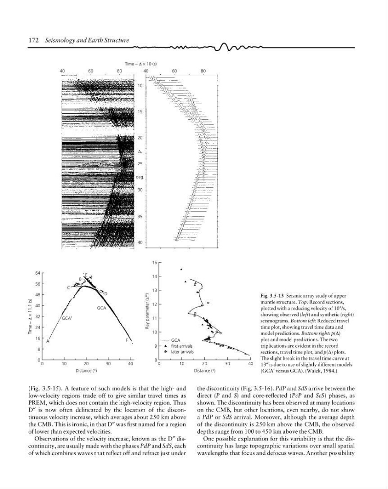
Fig. 3.5-13 Seismic array study of upper
mantle structure. Top: Record sections,
plotted with a reducing velocity of 10°/s,
showing observed (left) and synthetic (right)
seismograms. Bottom left: Reduced travel
time plot, showing travel time data and
model predictions. Bottom right: p(∆)
plot and model predictions. The two
triplications are evident in the record
sections, travel time plot, and p(∆) plots.
The slight break in the travel time curve at
13° is due to use of slightly different models
(GCA′ versus GCA). (Walck, 1984.)
Time
− ∆ × 11.1 (s)
64
56
48
40
32
24
16
8
0
0
1 0
2 0
3 0
4 0
Distance (°)
A
GCA′
GCA
F
D
C
B
E
40
15
14
13
12
11
10
9
8
Ray parameter (s/°)
30
20
10
0
Distance (°)
40
60
80
80
60
40
Time − ∆ × 10 (s)
10
15
20
∆,
25
deg.
30
35
40
GCA
first arrivals
later arrivals
(Fig. 3.5-15). A feature of such models is that the high- and
low-velocity regions trade off to give similar travel times as
PREM, which does not contain the high-velocity region. Thus
D″ is now often delineated by the location of the discontinuous velocity increase, which averages about 250 km above
the CMB. This is ironic, in that D″ was first named for a region
of lower than expected velocities.
Observations of the velocity increase, known as the D″ discontinuity, are usually made with the phases PdP and SdS, each
of which combines waves that reflect off and refract just under
the discontinuity (Fig. 3.5-16). PdP and SdS arrive between the
direct (P and S) and core-reflected (PcP and ScS) phases, as
shown. The discontinuity has been observed at many locations
on the CMB, but other locations, even nearby, do not show
a PdP or SdS arrival. Moreover, although the average depth
of the discontinuity is 250 km above the CMB, the observed
depths range from 100 to 450 km above the CMB.
One possible explanation for this variability is that the discontinuity has large topographic variations over small spatial
wavelengths that focus and defocus waves. Another possibility
Fig. 3.5-13 Seismic array study of upper
mantle structure. Top: Record sections,
plotted with a reducing velocity of 10°/s,
showing observed (left) and synthetic (right)
seismograms. Bottom left: Reduced travel
time plot, showing travel time data and
model predictions. Bottom right: p(∆)
plot and model predictions. The two
triplications are evident in the record
sections, travel time plot, and p(∆) plots.
The slight break in the travel time curve at
13° is due to use of slightly different models
(GCA′ versus GCA). (Walck, 1984.)