

3.5 Body wave travel time studies 171
8 The uncertainties about D″ have been illustrated by describing its thickness as
250 ± 250 km (Jeanloz, 1990).
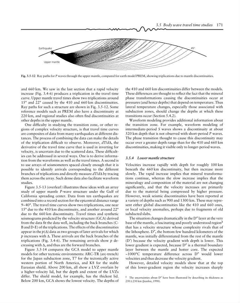
Fig. 3.5-12 Ray paths for P waves through the upper mantle, computed for earth model PREM, showing triplications due to mantle discontinuities.
Earthquake
Upper mantle
45°
and 660 km. We saw in the last section that a rapid velocity
increase (Fig. 3.4-6) produces a triplication in the travel time
curve. Upper mantle travel times show two triplications around
15° and 22° caused by the 410 and 660 km discontinuities.
Ray paths for such a structure are shown in Fig. 3.5-12. Some
reference models such as PREM also have a discontinuity at
220 km, and regional studies also often find discontinuities at
other depths in the upper mantle.
One difficulty in studying the transition zone, or other regions of complex velocity structure, is that travel time curves
are composites of data from many earthquakes at different distances. The process of combining the data can make the details
of the triplication difficult to observe. Moreover, dT/d∆, the
derivative of the travel time curve that is used in inverting for
velocity, is uncertain due to the scattered data. These difficulties can be addressed in several ways. One is to derive information from the waveforms as well as the travel times. A second is
to use arrays of seismometers spaced closely enough that it is
possible to identify arrivals corresponding to the different
branches of triplications and directly measure dT/d∆ by tracing
them across the array. Such dense data also facilitate waveform
studies.
Figure 3.5-13 (overleaf ) illustrates these ideas with an array
study of upper mantle P-wave structure under the Gulf of
California spreading center. Data from ten earthquakes are
combined into a record section for the epicentral distance range
9–40°. The travel time curves show two triplications, one near
15° due to the 410 km discontinuity, and another around 22°
due to the 660 km discontinuity. Travel times and synthetic
seismograms predicted by the velocity structure (GCA) derived
from the data fit the data well, including the back branches (CB and D-E) of the triplications. The effects of the discontinuities
appear in the p(∆) data as two groups of later arrivals for which
p increases with ∆. These arrivals are the back branches of the
triplications (Fig. 3.4-6). The remaining arrivals show p decreasing with ∆, and thus are the forward branches.
Figure 3.5-14 compares the GCA model to upper mantle
models for other tectonic environments: ARC-TR (arc-trench)
for the Japan subduction zone, T7 for the tectonically active
western portion of North America, and K8 for the stable
Eurasian shield. Above 200 km, all show a LVZ overlain by
a higher-velocity lid, but the depth and extent of the LVZs
differ. The shield model, for example, has the thickest lid.
Below 200 km, GCA shows the lowest velocity. The depths of
the 410 and 660 km discontinuities differ between the models.
These differences are thought to reflect the fact that the mineral
phase transformations causing the discontinuities occur at
pressures (and hence depths) that depend on temperature. Thus
lateral temperature changes, especially those associated with
subduction zones, should change the depths at which these
transitions occur (Section 5.4.2).
Waveform modeling provides additional information about
the transition zone. For example, waveform modeling of
intermediate-period S waves shows a discontinuity at about
520 km depth that is not observed with short-period P waves.
The phase transition thought to cause this discontinuity may
occur over a greater depth range than for the 410 and 660 km
discontinuities, making it visible only to longer-period waves.
3.5.4 Lower mantle structure
Velocities increase rapidly with depth for roughly 100 km
beneath the 660 km discontinuity, but then increase more
slowly. The rapid increase implies that mineral transformations continue, whereas the slow increase implies that the
mineralogy and composition of the material are not changing
significantly, and that the velocity increases are primarily
due to the material being compressed by higher pressure.
However, weak seismic discontinuities have been reported at
a variety of depths such as 900 and 1300 km. These may represent either global discontinuities like the 410 and 660 ones,
or local velocity anomalies, perhaps due to fragments of old
subducted slabs.
The situation changes dramatically in the D″ layer at the very
base of the mantle, a fascinating and poorly understood region 8
that has a velocity structure whose complexity rivals that of
the lithosphere. D″, the bottom few hundred kilometers of the
mantle, was initially differentiated from the rest of the mantle
(D′) because the velocity gradient with depth is lower. This
lower gradient is expected, because D″ is a thermal boundary
layer between the mantle and hotter core. The expected
~1000°C temperature difference across D″ would lower
velocities and thus decrease the velocity gradient.
However, detailed velocity models show that at the top
of this lower-gradient region the velocity increases sharply
8 The uncertainties about D″ have been illustrated by describing its thickness as
250 ± 250 km (Jeanloz, 1990).
Fig. 3.5-12 Ray paths for P waves through the upper mantle, computed for earth model PREM, showing triplications due to mantle discontinuities.
Earthquake
Upper mantle
45°
and 660 km. We saw in the last section that a rapid velocity
increase (Fig. 3.4-6) produces a triplication in the travel time
curve. Upper mantle travel times show two triplications around
15° and 22° caused by the 410 and 660 km discontinuities.
Ray paths for such a structure are shown in Fig. 3.5-12. Some
reference models such as PREM also have a discontinuity at
220 km, and regional studies also often find discontinuities at
other depths in the upper mantle.
One difficulty in studying the transition zone, or other regions of complex velocity structure, is that travel time curves
are composites of data from many earthquakes at different distances. The process of combining the data can make the details
of the triplication difficult to observe. Moreover, dT/d∆, the
derivative of the travel time curve that is used in inverting for
velocity, is uncertain due to the scattered data. These difficulties can be addressed in several ways. One is to derive information from the waveforms as well as the travel times. A second is
to use arrays of seismometers spaced closely enough that it is
possible to identify arrivals corresponding to the different
branches of triplications and directly measure dT/d∆ by tracing
them across the array. Such dense data also facilitate waveform
studies.
Figure 3.5-13 (overleaf ) illustrates these ideas with an array
study of upper mantle P-wave structure under the Gulf of
California spreading center. Data from ten earthquakes are
combined into a record section for the epicentral distance range
9–40°. The travel time curves show two triplications, one near
15° due to the 410 km discontinuity, and another around 22°
due to the 660 km discontinuity. Travel times and synthetic
seismograms predicted by the velocity structure (GCA) derived
from the data fit the data well, including the back branches (CB and D-E) of the triplications. The effects of the discontinuities
appear in the p(∆) data as two groups of later arrivals for which
p increases with ∆. These arrivals are the back branches of the
triplications (Fig. 3.4-6). The remaining arrivals show p decreasing with ∆, and thus are the forward branches.
Figure 3.5-14 compares the GCA model to upper mantle
models for other tectonic environments: ARC-TR (arc-trench)
for the Japan subduction zone, T7 for the tectonically active
western portion of North America, and K8 for the stable
Eurasian shield. Above 200 km, all show a LVZ overlain by
a higher-velocity lid, but the depth and extent of the LVZs
differ. The shield model, for example, has the thickest lid.
Below 200 km, GCA shows the lowest velocity. The depths of
the 410 and 660 km discontinuities differ between the models.
These differences are thought to reflect the fact that the mineral
phase transformations causing the discontinuities occur at
pressures (and hence depths) that depend on temperature. Thus
lateral temperature changes, especially those associated with
subduction zones, should change the depths at which these
transitions occur (Section 5.4.2).
Waveform modeling provides additional information about
the transition zone. For example, waveform modeling of
intermediate-period S waves shows a discontinuity at about
520 km depth that is not observed with short-period P waves.
The phase transition thought to cause this discontinuity may
occur over a greater depth range than for the 410 and 660 km
discontinuities, making it visible only to longer-period waves.
3.5.4 Lower mantle structure
Velocities increase rapidly with depth for roughly 100 km
beneath the 660 km discontinuity, but then increase more
slowly. The rapid increase implies that mineral transformations continue, whereas the slow increase implies that the
mineralogy and composition of the material are not changing
significantly, and that the velocity increases are primarily
due to the material being compressed by higher pressure.
However, weak seismic discontinuities have been reported at
a variety of depths such as 900 and 1300 km. These may represent either global discontinuities like the 410 and 660 ones,
or local velocity anomalies, perhaps due to fragments of old
subducted slabs.
The situation changes dramatically in the D″ layer at the very
base of the mantle, a fascinating and poorly understood region 8
that has a velocity structure whose complexity rivals that of
the lithosphere. D″, the bottom few hundred kilometers of the
mantle, was initially differentiated from the rest of the mantle
(D′) because the velocity gradient with depth is lower. This
lower gradient is expected, because D″ is a thermal boundary
layer between the mantle and hotter core. The expected
~1000°C temperature difference across D″ would lower
velocities and thus decrease the velocity gradient.
However, detailed velocity models show that at the top
of this lower-gradient region the velocity increases sharply