

0
10
20
30
40
50
60
70
S
ScS
sS,SS
sScS,S3,S4
ScS 2 sScS 2
ScS 3 sScS 3
ScS 4 sScS 4
Minutes after the earthquake
Seismometer
Deep
earthquake
ScS
ScS 2
ScS 3
ScS 4
sScS
sS
SS
S
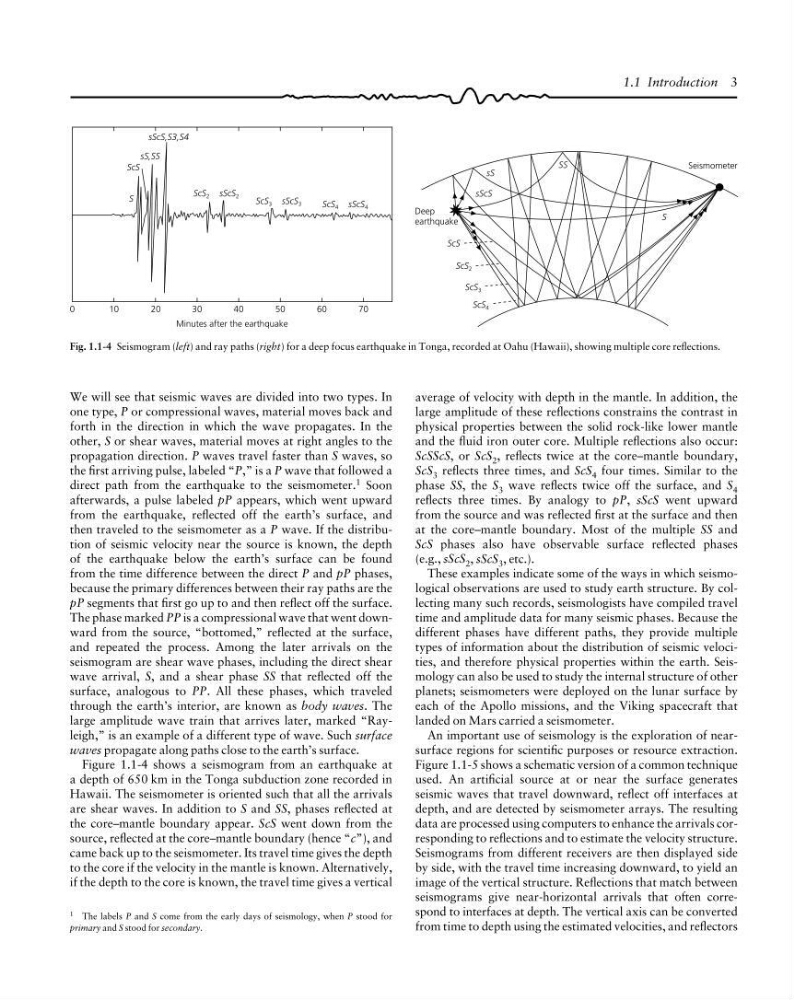
Fig. 1.1-4 Seismogram (left) and ray paths (right) for a deep focus earthquake in Tonga, recorded at Oahu (Hawaii), showing multiple core reflections.
1 The labels P and S come from the early days of seismology, when P stood for
primary and S stood for secondary.
average of velocity with depth in the mantle. In addition, the
large amplitude of these reflections constrains the contrast in
physical properties between the solid rock-like lower mantle
and the fluid iron outer core. Multiple reflections also occur:
ScSScS, or ScS 2 , reflects twice at the core–mantle boundary,
ScS 3 reflects three times, and ScS 4 four times. Similar to the
phase SS, the S 3 wave reflects twice off the surface, and S 4
reflects three times. By analogy to pP, sScS went upward
from the source and was reflected first at the surface and then
at the core–mantle boundary. Most of the multiple SS and
ScS phases also have observable surface reflected phases
(e.g., sScS 2 , sScS 3 , etc.).
These examples indicate some of the ways in which seismological observations are used to study earth structure. By collecting many such records, seismologists have compiled travel
time and amplitude data for many seismic phases. Because the
different phases have different paths, they provide multiple
types of information about the distribution of seismic velocities, and therefore physical properties within the earth. Seismology can also be used to study the internal structure of other
planets; seismometers were deployed on the lunar surface by
each of the Apollo missions, and the Viking spacecraft that
landed on Mars carried a seismometer.
An important use of seismology is the exploration of nearsurface regions for scientific purposes or resource extraction.
Figure 1.1-5 shows a schematic version of a common technique
used. An artificial source at or near the surface generates
seismic waves that travel downward, reflect off interfaces at
depth, and are detected by seismometer arrays. The resulting
data are processed using computers to enhance the arrivals corresponding to reflections and to estimate the velocity structure.
Seismograms from different receivers are then displayed side
by side, with the travel time increasing downward, to yield an
image of the vertical structure. Reflections that match between
seismograms give near-horizontal arrivals that often correspond to interfaces at depth. The vertical axis can be converted
from time to depth using the estimated velocities, and reflectors
We will see that seismic waves are divided into two types. In
one type, P or compressional waves, material moves back and
forth in the direction in which the wave propagates. In the
other, S or shear waves, material moves at right angles to the
propagation direction. P waves travel faster than S waves, so
the first arriving pulse, labeled “P,” is a P wave that followed a
direct path from the earthquake to the seismometer. 1 Soon
afterwards, a pulse labeled pP appears, which went upward
from the earthquake, reflected off the earth’s surface, and
then traveled to the seismometer as a P wave. If the distribution of seismic velocity near the source is known, the depth
of the earthquake below the earth’s surface can be found
from the time difference between the direct P and pP phases,
because the primary differences between their ray paths are the
pP segments that first go up to and then reflect off the surface.
The phase marked PP is a compressional wave that went downward from the source, “bottomed,” reflected at the surface,
and repeated the process. Among the later arrivals on the
seismogram are shear wave phases, including the direct shear
wave arrival, S, and a shear phase SS that reflected off the
surface, analogous to PP. All these phases, which traveled
through the earth’s interior, are known as body waves. The
large amplitude wave train that arrives later, marked “Rayleigh,” is an example of a different type of wave. Such surface
waves propagate along paths close to the earth’s surface.
Figure 1.1-4 shows a seismogram from an earthquake at
a depth of 650 km in the Tonga subduction zone recorded in
Hawaii. The seismometer is oriented such that all the arrivals
are shear waves. In addition to S and SS, phases reflected at
the core–mantle boundary appear. ScS went down from the
source, reflected at the core–mantle boundary (hence “c”), and
came back up to the seismometer. Its travel time gives the depth
to the core if the velocity in the mantle is known. Alternatively,
if the depth to the core is known, the travel time gives a vertical
1.1 Introduction 3
10
20
30
40
50
60
70
S
ScS
sS,SS
sScS,S3,S4
ScS 2 sScS 2
ScS 3 sScS 3
ScS 4 sScS 4
Minutes after the earthquake
Seismometer
Deep
earthquake
ScS
ScS 2
ScS 3
ScS 4
sScS
sS
SS
S
Fig. 1.1-4 Seismogram (left) and ray paths (right) for a deep focus earthquake in Tonga, recorded at Oahu (Hawaii), showing multiple core reflections.
1 The labels P and S come from the early days of seismology, when P stood for
primary and S stood for secondary.
average of velocity with depth in the mantle. In addition, the
large amplitude of these reflections constrains the contrast in
physical properties between the solid rock-like lower mantle
and the fluid iron outer core. Multiple reflections also occur:
ScSScS, or ScS 2 , reflects twice at the core–mantle boundary,
ScS 3 reflects three times, and ScS 4 four times. Similar to the
phase SS, the S 3 wave reflects twice off the surface, and S 4
reflects three times. By analogy to pP, sScS went upward
from the source and was reflected first at the surface and then
at the core–mantle boundary. Most of the multiple SS and
ScS phases also have observable surface reflected phases
(e.g., sScS 2 , sScS 3 , etc.).
These examples indicate some of the ways in which seismological observations are used to study earth structure. By collecting many such records, seismologists have compiled travel
time and amplitude data for many seismic phases. Because the
different phases have different paths, they provide multiple
types of information about the distribution of seismic velocities, and therefore physical properties within the earth. Seismology can also be used to study the internal structure of other
planets; seismometers were deployed on the lunar surface by
each of the Apollo missions, and the Viking spacecraft that
landed on Mars carried a seismometer.
An important use of seismology is the exploration of nearsurface regions for scientific purposes or resource extraction.
Figure 1.1-5 shows a schematic version of a common technique
used. An artificial source at or near the surface generates
seismic waves that travel downward, reflect off interfaces at
depth, and are detected by seismometer arrays. The resulting
data are processed using computers to enhance the arrivals corresponding to reflections and to estimate the velocity structure.
Seismograms from different receivers are then displayed side
by side, with the travel time increasing downward, to yield an
image of the vertical structure. Reflections that match between
seismograms give near-horizontal arrivals that often correspond to interfaces at depth. The vertical axis can be converted
from time to depth using the estimated velocities, and reflectors
We will see that seismic waves are divided into two types. In
one type, P or compressional waves, material moves back and
forth in the direction in which the wave propagates. In the
other, S or shear waves, material moves at right angles to the
propagation direction. P waves travel faster than S waves, so
the first arriving pulse, labeled “P,” is a P wave that followed a
direct path from the earthquake to the seismometer. 1 Soon
afterwards, a pulse labeled pP appears, which went upward
from the earthquake, reflected off the earth’s surface, and
then traveled to the seismometer as a P wave. If the distribution of seismic velocity near the source is known, the depth
of the earthquake below the earth’s surface can be found
from the time difference between the direct P and pP phases,
because the primary differences between their ray paths are the
pP segments that first go up to and then reflect off the surface.
The phase marked PP is a compressional wave that went downward from the source, “bottomed,” reflected at the surface,
and repeated the process. Among the later arrivals on the
seismogram are shear wave phases, including the direct shear
wave arrival, S, and a shear phase SS that reflected off the
surface, analogous to PP. All these phases, which traveled
through the earth’s interior, are known as body waves. The
large amplitude wave train that arrives later, marked “Rayleigh,” is an example of a different type of wave. Such surface
waves propagate along paths close to the earth’s surface.
Figure 1.1-4 shows a seismogram from an earthquake at
a depth of 650 km in the Tonga subduction zone recorded in
Hawaii. The seismometer is oriented such that all the arrivals
are shear waves. In addition to S and SS, phases reflected at
the core–mantle boundary appear. ScS went down from the
source, reflected at the core–mantle boundary (hence “c”), and
came back up to the seismometer. Its travel time gives the depth
to the core if the velocity in the mantle is known. Alternatively,
if the depth to the core is known, the travel time gives a vertical
1.1 Introduction 3