

sP
pP
pPP
S
Rayleigh
SS/ScS
sS
PcS
PP/PcP
P
0
5
10
15
Time (min)
Rayleigh
pPP
Receiver
PP
ScS
PcS
Core
Mantle
P wave
S wave
Surface
wave
Earthquake
sP
pP
S
P
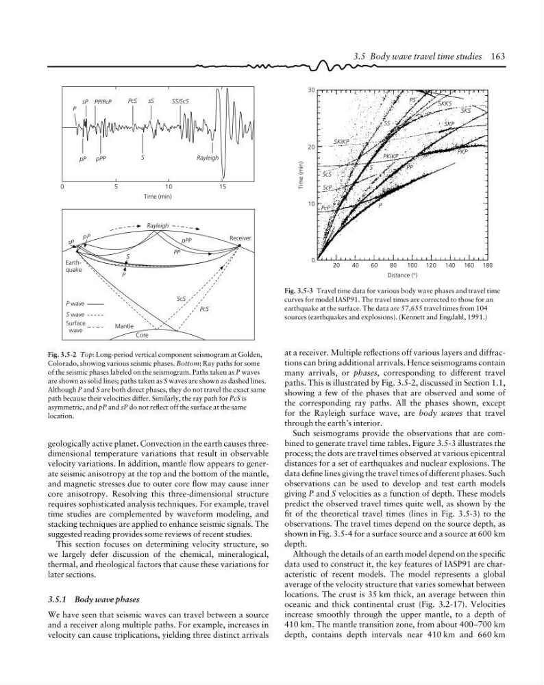
Fig. 3.5-3 Travel time data for various body wave phases and travel time
curves for model IASP91. The travel times are corrected to those for an
earthquake at the surface. The data are 57,655 travel times from 104
sources (earthquakes and explosions). (Kennett and Engdahl, 1991.)
PKP
Time (min)
30
SKiKP
ScS
ScP
PcP
P
S
PP
PKiKP
SS
PS
SKP
SKKS
SKS
20
Distance (°)
20
10
0
40
60
80
100 120 140 160 180
at a receiver. Multiple reflections off various layers and diffractions can bring additional arrivals. Hence seismograms contain
many arrivals, or phases, corresponding to different travel
paths. This is illustrated by Fig. 3.5-2, discussed in Section 1.1,
showing a few of the phases that are observed and some of
the corresponding ray paths. All the phases shown, except
for the Rayleigh surface wave, are body waves that travel
through the earth’s interior.
Such seismograms provide the observations that are combined to generate travel time tables. Figure 3.5-3 illustrates the
process; the dots are travel times observed at various epicentral
distances for a set of earthquakes and nuclear explosions. The
data define lines giving the travel times of different phases. Such
observations can be used to develop and test earth models
giving P and S velocities as a function of depth. These models
predict the observed travel times quite well, as shown by the
fit of the theoretical travel times (lines in Fig. 3.5-3) to the
observations. The travel times depend on the source depth, as
shown in Fig. 3.5-4 for a surface source and a source at 600 km
depth.
Although the details of an earth model depend on the specific
data used to construct it, the key features of IASP91 are characteristic of recent models. The model represents a global
average of the velocity structure that varies somewhat between
locations. The crust is 35 km thick, an average between thin
oceanic and thick continental crust (Fig. 3.2-17). Velocities
increase smoothly through the upper mantle, to a depth of
410 km. The mantle transition zone, from about 400–700 km
depth, contains depth intervals near 410 km and 660 km
3.5 Body wave travel time studies 163
geologically active planet. Convection in the earth causes threedimensional temperature variations that result in observable
velocity variations. In addition, mantle flow appears to generate seismic anisotropy at the top and the bottom of the mantle,
and magnetic stresses due to outer core flow may cause inner
core anisotropy. Resolving this three-dimensional structure
requires sophisticated analysis techniques. For example, travel
time studies are complemented by waveform modeling, and
stacking techniques are applied to enhance seismic signals. The
suggested reading provides some reviews of recent studies.
This section focuses on determining velocity structure, so
we largely defer discussion of the chemical, mineralogical,
thermal, and rheological factors that cause these variations for
later sections.
3.5.1 Body wave phases
We have seen that seismic waves can travel between a source
and a receiver along multiple paths. For example, increases in
velocity can cause triplications, yielding three distinct arrivals
Fig. 3.5-2 Top: Long-period vertical component seismogram at Golden,
Colorado, showing various seismic phases. Bottom: Ray paths for some
of the seismic phases labeled on the seismogram. Paths taken as P waves
are shown as solid lines; paths taken as S waves are shown as dashed lines.
Although P and S are both direct phases, they do not travel the exact same
path because their velocities differ. Similarly, the ray path for PcS is
asymmetric, and pP and sP do not reflect off the surface at the same
location.
pP
pPP
S
Rayleigh
SS/ScS
sS
PcS
PP/PcP
P
0
5
10
15
Time (min)
Rayleigh
pPP
Receiver
PP
ScS
PcS
Core
Mantle
P wave
S wave
Surface
wave
Earthquake
sP
pP
S
P
Fig. 3.5-3 Travel time data for various body wave phases and travel time
curves for model IASP91. The travel times are corrected to those for an
earthquake at the surface. The data are 57,655 travel times from 104
sources (earthquakes and explosions). (Kennett and Engdahl, 1991.)
PKP
Time (min)
30
SKiKP
ScS
ScP
PcP
P
S
PP
PKiKP
SS
PS
SKP
SKKS
SKS
20
Distance (°)
20
10
0
40
60
80
100 120 140 160 180
at a receiver. Multiple reflections off various layers and diffractions can bring additional arrivals. Hence seismograms contain
many arrivals, or phases, corresponding to different travel
paths. This is illustrated by Fig. 3.5-2, discussed in Section 1.1,
showing a few of the phases that are observed and some of
the corresponding ray paths. All the phases shown, except
for the Rayleigh surface wave, are body waves that travel
through the earth’s interior.
Such seismograms provide the observations that are combined to generate travel time tables. Figure 3.5-3 illustrates the
process; the dots are travel times observed at various epicentral
distances for a set of earthquakes and nuclear explosions. The
data define lines giving the travel times of different phases. Such
observations can be used to develop and test earth models
giving P and S velocities as a function of depth. These models
predict the observed travel times quite well, as shown by the
fit of the theoretical travel times (lines in Fig. 3.5-3) to the
observations. The travel times depend on the source depth, as
shown in Fig. 3.5-4 for a surface source and a source at 600 km
depth.
Although the details of an earth model depend on the specific
data used to construct it, the key features of IASP91 are characteristic of recent models. The model represents a global
average of the velocity structure that varies somewhat between
locations. The crust is 35 km thick, an average between thin
oceanic and thick continental crust (Fig. 3.2-17). Velocities
increase smoothly through the upper mantle, to a depth of
410 km. The mantle transition zone, from about 400–700 km
depth, contains depth intervals near 410 km and 660 km
3.5 Body wave travel time studies 163
geologically active planet. Convection in the earth causes threedimensional temperature variations that result in observable
velocity variations. In addition, mantle flow appears to generate seismic anisotropy at the top and the bottom of the mantle,
and magnetic stresses due to outer core flow may cause inner
core anisotropy. Resolving this three-dimensional structure
requires sophisticated analysis techniques. For example, travel
time studies are complemented by waveform modeling, and
stacking techniques are applied to enhance seismic signals. The
suggested reading provides some reviews of recent studies.
This section focuses on determining velocity structure, so
we largely defer discussion of the chemical, mineralogical,
thermal, and rheological factors that cause these variations for
later sections.
3.5.1 Body wave phases
We have seen that seismic waves can travel between a source
and a receiver along multiple paths. For example, increases in
velocity can cause triplications, yielding three distinct arrivals
Fig. 3.5-2 Top: Long-period vertical component seismogram at Golden,
Colorado, showing various seismic phases. Bottom: Ray paths for some
of the seismic phases labeled on the seismogram. Paths taken as P waves
are shown as solid lines; paths taken as S waves are shown as dashed lines.
Although P and S are both direct phases, they do not travel the exact same
path because their velocities differ. Similarly, the ray path for PcS is
asymmetric, and pP and sP do not reflect off the surface at the same
location.