

162 Seismology and Earth Structure
the outer radius of the low-velocity zone, substituted for r p , to
find the distance and time the ray traveled on its way down to
the low-velocity zone. Subtracting these from the known T(∆)
curve gives a T ′(∆) curve for a “mini-earth” with radius r′.
Because in this “mini-earth” the velocity increases with depth,
the Herglotz–Wiechert method is applied again.
3.5 Body wave travel time studies
We saw in the last section that travel time data can be used
to determine seismic velocity as a function of depth. Beginning early in the 1900s, travel time tables were compiled by
combining data from many earthquakes observed at various
epicentral distances. These seismological observations provide
the primary data for our view of the basic features of the earth’s
velocity structure. This picture, an essentially layered earth
composed of a thin crust, a mantle, a liquid outer core, and
a solid inner core, is key to our thinking about how the earth
evolved and operates. This concept was largely developed by
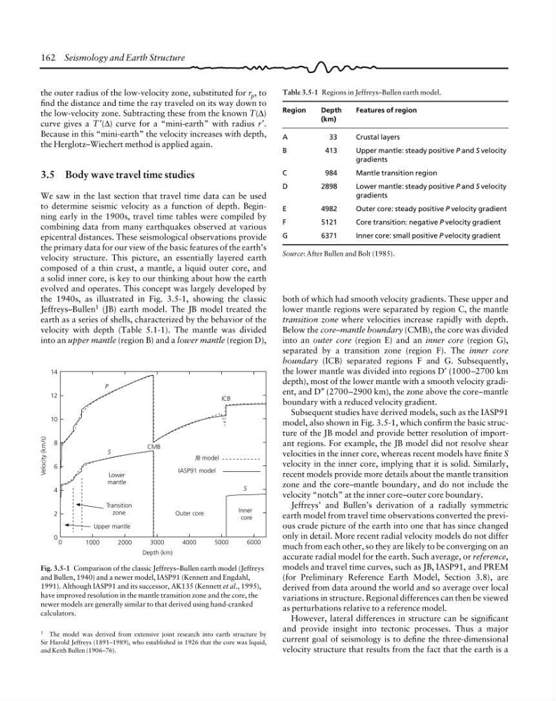
the 1940s, as illustrated in Fig. 3.5-1, showing the classic
Jeffreys–Bullen 1 (JB) earth model. The JB model treated the
earth as a series of shells, characterized by the behavior of the
velocity with depth (Table 5.1-1). The mantle was divided
into an upper mantle (region B) and a lower mantle (region D),
Table 3.5-1 Regions in Jeffreys–Bullen earth model.
Region
Depth
Features of region
(km)
A
33
Crustal layers
B
413
Upper mantle: steady positive P and S velocity
gradients
C
984
Mantle transition region
D
2898
Lower mantle: steady positive P and S velocity
gradients
E
4982
Outer core: steady positive P velocity gradient
F
5121
Core transition: negative P velocity gradient
G
6371
Inner core: small positive P velocity gradient
Source: After Bullen and Bolt (1985).
1 The model was derived from extensive joint research into earth structure by
Sir Harold Jeffreys (1891–1989), who established in 1926 that the core was liquid,
and Keith Bullen (1906–76).
Fig. 3.5-1 Comparison of the classic Jeffreys–Bullen earth model (Jeffreys
and Bullen, 1940) and a newer model, IASP91 (Kennett and Engdahl,
1991). Although IASP91 and its successor, AK135 (Kennett et al., 1995),
have improved resolution in the mantle transition zone and the core, the
newer models are generally similar to that derived using hand-cranked
calculators.
ICB
Velocity (km/s)
14
12
10
8
6
4
2
0
Outer core
0
1000
2000
3000
4000
5000
6000
Depth (km)
Inner
core
JB model
IASP91 model
S
CMB
S
Lower
mantle
Transition
zone
Upper mantle
P
both of which had smooth velocity gradients. These upper and
lower mantle regions were separated by region C, the mantle
transition zone where velocities increase rapidly with depth.
Below the core–mantle boundary (CMB), the core was divided
into an outer core (region E) and an inner core (region G),
separated by a transition zone (region F). The inner core
boundary (ICB) separated regions F and G. Subsequently,
the lower mantle was divided into regions D′ (1000–2700 km
depth), most of the lower mantle with a smooth velocity gradient, and D″ (2700–2900 km), the zone above the core–mantle
boundary with a reduced velocity gradient.
Subsequent studies have derived models, such as the IASP91
model, also shown in Fig. 3.5-1, which confirm the basic structure of the JB model and provide better resolution of important regions. For example, the JB model did not resolve shear
velocities in the inner core, whereas recent models have finite S
velocity in the inner core, implying that it is solid. Similarly,
recent models provide more details about the mantle transition
zone and the core–mantle boundary, and do not include the
velocity “notch” at the inner core–outer core boundary.
Jeffreys’ and Bullen’s derivation of a radially symmetric
earth model from travel time observations converted the previous crude picture of the earth into one that has since changed
only in detail. More recent radial velocity models do not differ
much from each other, so they are likely to be converging on an
accurate radial model for the earth. Such average, or reference,
models and travel time curves, such as JB, IASP91, and PREM
(for Preliminary Reference Earth Model, Section 3.8), are
derived from data around the world and so average over local
variations in structure. Regional differences can then be viewed
as perturbations relative to a reference model.
However, lateral differences in structure can be significant
and provide insight into tectonic processes. Thus a major
current goal of seismology is to define the three-dimensional
velocity structure that results from the fact that the earth is a
the outer radius of the low-velocity zone, substituted for r p , to
find the distance and time the ray traveled on its way down to
the low-velocity zone. Subtracting these from the known T(∆)
curve gives a T ′(∆) curve for a “mini-earth” with radius r′.
Because in this “mini-earth” the velocity increases with depth,
the Herglotz–Wiechert method is applied again.
3.5 Body wave travel time studies
We saw in the last section that travel time data can be used
to determine seismic velocity as a function of depth. Beginning early in the 1900s, travel time tables were compiled by
combining data from many earthquakes observed at various
epicentral distances. These seismological observations provide
the primary data for our view of the basic features of the earth’s
velocity structure. This picture, an essentially layered earth
composed of a thin crust, a mantle, a liquid outer core, and
a solid inner core, is key to our thinking about how the earth
evolved and operates. This concept was largely developed by
the 1940s, as illustrated in Fig. 3.5-1, showing the classic
Jeffreys–Bullen 1 (JB) earth model. The JB model treated the
earth as a series of shells, characterized by the behavior of the
velocity with depth (Table 5.1-1). The mantle was divided
into an upper mantle (region B) and a lower mantle (region D),
Table 3.5-1 Regions in Jeffreys–Bullen earth model.
Region
Depth
Features of region
(km)
A
33
Crustal layers
B
413
Upper mantle: steady positive P and S velocity
gradients
C
984
Mantle transition region
D
2898
Lower mantle: steady positive P and S velocity
gradients
E
4982
Outer core: steady positive P velocity gradient
F
5121
Core transition: negative P velocity gradient
G
6371
Inner core: small positive P velocity gradient
Source: After Bullen and Bolt (1985).
1 The model was derived from extensive joint research into earth structure by
Sir Harold Jeffreys (1891–1989), who established in 1926 that the core was liquid,
and Keith Bullen (1906–76).
Fig. 3.5-1 Comparison of the classic Jeffreys–Bullen earth model (Jeffreys
and Bullen, 1940) and a newer model, IASP91 (Kennett and Engdahl,
1991). Although IASP91 and its successor, AK135 (Kennett et al., 1995),
have improved resolution in the mantle transition zone and the core, the
newer models are generally similar to that derived using hand-cranked
calculators.
ICB
Velocity (km/s)
14
12
10
8
6
4
2
0
Outer core
0
1000
2000
3000
4000
5000
6000
Depth (km)
Inner
core
JB model
IASP91 model
S
CMB
S
Lower
mantle
Transition
zone
Upper mantle
P
both of which had smooth velocity gradients. These upper and
lower mantle regions were separated by region C, the mantle
transition zone where velocities increase rapidly with depth.
Below the core–mantle boundary (CMB), the core was divided
into an outer core (region E) and an inner core (region G),
separated by a transition zone (region F). The inner core
boundary (ICB) separated regions F and G. Subsequently,
the lower mantle was divided into regions D′ (1000–2700 km
depth), most of the lower mantle with a smooth velocity gradient, and D″ (2700–2900 km), the zone above the core–mantle
boundary with a reduced velocity gradient.
Subsequent studies have derived models, such as the IASP91
model, also shown in Fig. 3.5-1, which confirm the basic structure of the JB model and provide better resolution of important regions. For example, the JB model did not resolve shear
velocities in the inner core, whereas recent models have finite S
velocity in the inner core, implying that it is solid. Similarly,
recent models provide more details about the mantle transition
zone and the core–mantle boundary, and do not include the
velocity “notch” at the inner core–outer core boundary.
Jeffreys’ and Bullen’s derivation of a radially symmetric
earth model from travel time observations converted the previous crude picture of the earth into one that has since changed
only in detail. More recent radial velocity models do not differ
much from each other, so they are likely to be converging on an
accurate radial model for the earth. Such average, or reference,
models and travel time curves, such as JB, IASP91, and PREM
(for Preliminary Reference Earth Model, Section 3.8), are
derived from data around the world and so average over local
variations in structure. Regional differences can then be viewed
as perturbations relative to a reference model.
However, lateral differences in structure can be significant
and provide insight into tectonic processes. Thus a major
current goal of seismology is to define the three-dimensional
velocity structure that results from the fact that the earth is a