

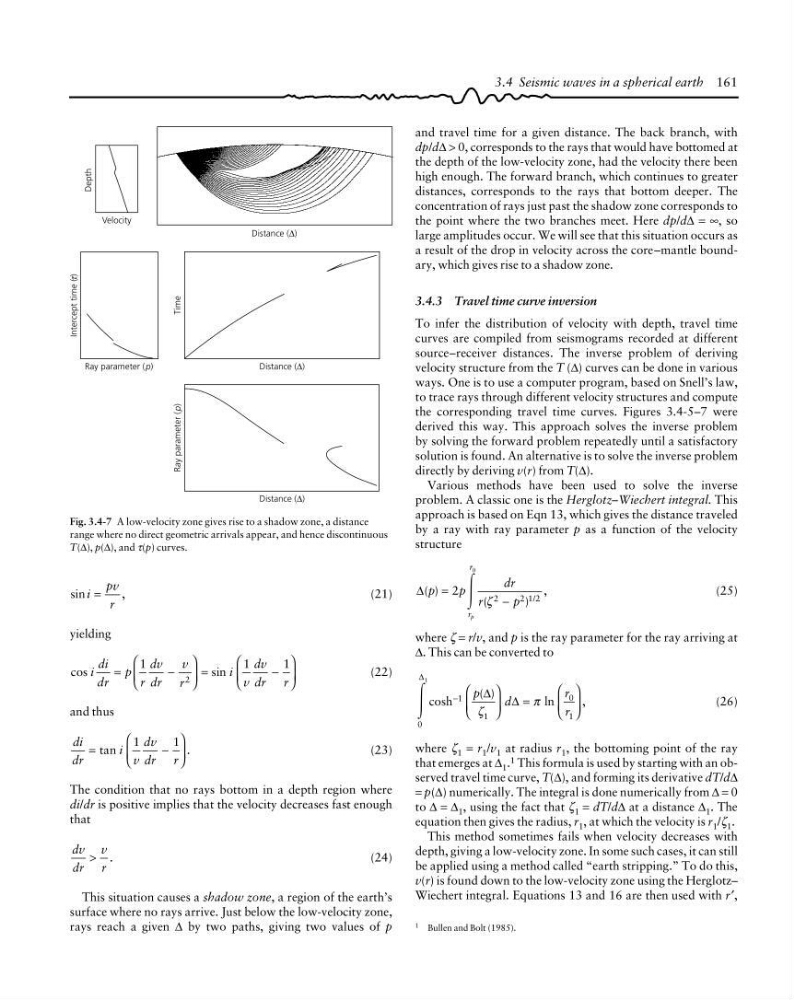
and travel time for a given distance. The back branch, with
dp/d∆ > 0, corresponds to the rays that would have bottomed at
the depth of the low-velocity zone, had the velocity there been
high enough. The forward branch, which continues to greater
distances, corresponds to the rays that bottom deeper. The
concentration of rays just past the shadow zone corresponds to
the point where the two branches meet. Here dp/d∆ = ∞, so
large amplitudes occur. We will see that this situation occurs as
a result of the drop in velocity across the core–mantle boundary, which gives rise to a shadow zone.
3.4.3 Travel time curve inversion
To infer the distribution of velocity with depth, travel time
curves are compiled from seismograms recorded at different
source–receiver distances. The inverse problem of deriving
velocity structure from the T (∆) curves can be done in various
ways. One is to use a computer program, based on Snell’s law,
to trace rays through different velocity structures and compute
the corresponding travel time curves. Figures 3.4-5–7 were
derived this way. This approach solves the inverse problem
by solving the forward problem repeatedly until a satisfactory
solution is found. An alternative is to solve the inverse problem
directly by deriving v(r) from T(∆).
Various methods have been used to solve the inverse
problem. A classic one is the Herglotz–Wiechert integral. This
approach is based on Eqn 13, which gives the distance traveled
by a ray with ray parameter p as a function of the velocity
structure
∆( )
(
)
,
/
p
p
dr
r
p
r
r
p
=
−
2
0
2
212
Ύ ζ
(25)
where ζ = r/v, and p is the ray parameter for the ray arriving at
∆. This can be converted to
Ύ
0
1
1
0
1
1
∆
∆
∆
cosh
( )
ln
,
−
⎛
⎝
⎜
⎞
⎠
⎟
=
⎛
⎝
⎜
⎞
⎠
⎟
p
d
r
r
ζ
π
(26)
where ζ 1 = r 1 /v 1 at radius r 1 , the bottoming point of the ray
that emerges at ∆ 1 . 1 This formula is used by starting with an observed travel time curve, T(∆), and forming its derivative dT/d∆
= p(∆) numerically. The integral is done numerically from ∆ = 0
to ∆ = ∆ 1 , using the fact that ζ 1 = dT/d∆ at a distance ∆ 1 . The
equation then gives the radius, r 1 , at which the velocity is r 1 /ζ 1 .
This method sometimes fails when velocity decreases with
depth, giving a low-velocity zone. In some such cases, it can still
be applied using a method called “earth stripping.” To do this,
v(r) is found down to the low-velocity zone using the Herglotz–
Wiechert integral. Equations 13 and 16 are then used with r′,
3.4 Seismic waves in a spherical earth 161
Velocity
Depth
Distance (∆)
Time
Ray parameter (p)
Distance (∆)
Distance (∆)
Ray parameter (p)
Intercept time ( )
τ
Fig. 3.4-7 A low-velocity zone gives rise to a shadow zone, a distance
range where no direct geometric arrivals appear, and hence discontinuous
T(∆), p(∆), and τ(p) curves.
sin
,
i
pv
r
=
(21)
yielding
cos
sin
i
di
dr
p
r
dv
dr
v
r
i
v
dv
dr r
=
−
⎛
⎝
⎜
⎞
⎠
⎟ =
−
⎛
⎝
⎜
⎞
⎠
⎟
1
1
1
2
(22)
and thus
di
dr
i
v
dv
dr r
tan
.
=
−
⎛
⎝
⎜
⎞
⎠
⎟
1
1
(23)
The condition that no rays bottom in a depth region where
di/dr is positive implies that the velocity decreases fast enough
that
dv
dr
v
r
.
>
(24)
This situation causes a shadow zone, a region of the earth’s
surface where no rays arrive. Just below the low-velocity zone,
rays reach a given ∆ by two paths, giving two values of p
1 Bullen and Bolt (1985).
dp/d∆ > 0, corresponds to the rays that would have bottomed at
the depth of the low-velocity zone, had the velocity there been
high enough. The forward branch, which continues to greater
distances, corresponds to the rays that bottom deeper. The
concentration of rays just past the shadow zone corresponds to
the point where the two branches meet. Here dp/d∆ = ∞, so
large amplitudes occur. We will see that this situation occurs as
a result of the drop in velocity across the core–mantle boundary, which gives rise to a shadow zone.
3.4.3 Travel time curve inversion
To infer the distribution of velocity with depth, travel time
curves are compiled from seismograms recorded at different
source–receiver distances. The inverse problem of deriving
velocity structure from the T (∆) curves can be done in various
ways. One is to use a computer program, based on Snell’s law,
to trace rays through different velocity structures and compute
the corresponding travel time curves. Figures 3.4-5–7 were
derived this way. This approach solves the inverse problem
by solving the forward problem repeatedly until a satisfactory
solution is found. An alternative is to solve the inverse problem
directly by deriving v(r) from T(∆).
Various methods have been used to solve the inverse
problem. A classic one is the Herglotz–Wiechert integral. This
approach is based on Eqn 13, which gives the distance traveled
by a ray with ray parameter p as a function of the velocity
structure
∆( )
(
)
,
/
p
p
dr
r
p
r
r
p
=
−
2
0
2
212
Ύ ζ
(25)
where ζ = r/v, and p is the ray parameter for the ray arriving at
∆. This can be converted to
Ύ
0
1
1
0
1
1
∆
∆
∆
cosh
( )
ln
,
−
⎛
⎝
⎜
⎞
⎠
⎟
=
⎛
⎝
⎜
⎞
⎠
⎟
p
d
r
r
ζ
π
(26)
where ζ 1 = r 1 /v 1 at radius r 1 , the bottoming point of the ray
that emerges at ∆ 1 . 1 This formula is used by starting with an observed travel time curve, T(∆), and forming its derivative dT/d∆
= p(∆) numerically. The integral is done numerically from ∆ = 0
to ∆ = ∆ 1 , using the fact that ζ 1 = dT/d∆ at a distance ∆ 1 . The
equation then gives the radius, r 1 , at which the velocity is r 1 /ζ 1 .
This method sometimes fails when velocity decreases with
depth, giving a low-velocity zone. In some such cases, it can still
be applied using a method called “earth stripping.” To do this,
v(r) is found down to the low-velocity zone using the Herglotz–
Wiechert integral. Equations 13 and 16 are then used with r′,
3.4 Seismic waves in a spherical earth 161
Velocity
Depth
Distance (∆)
Time
Ray parameter (p)
Distance (∆)
Distance (∆)
Ray parameter (p)
Intercept time ( )
τ
Fig. 3.4-7 A low-velocity zone gives rise to a shadow zone, a distance
range where no direct geometric arrivals appear, and hence discontinuous
T(∆), p(∆), and τ(p) curves.
sin
,
i
pv
r
=
(21)
yielding
cos
sin
i
di
dr
p
r
dv
dr
v
r
i
v
dv
dr r
=
−
⎛
⎝
⎜
⎞
⎠
⎟ =
−
⎛
⎝
⎜
⎞
⎠
⎟
1
1
1
2
(22)
and thus
di
dr
i
v
dv
dr r
tan
.
=
−
⎛
⎝
⎜
⎞
⎠
⎟
1
1
(23)
The condition that no rays bottom in a depth region where
di/dr is positive implies that the velocity decreases fast enough
that
dv
dr
v
r
.
>
(24)
This situation causes a shadow zone, a region of the earth’s
surface where no rays arrive. Just below the low-velocity zone,
rays reach a given ∆ by two paths, giving two values of p
1 Bullen and Bolt (1985).